(Concept Review/Generative Models) Latent/Stable Diffusion Fully Explained, Part 4
Table of Contents:
Latent/Stable Diffusion Fully Explained! (Part 1)
-
Introduction
-
Stable Diffusion vs GAN
Latent/Stable Diffusion Fully Explained! (Part 2)
-
Motivation
-
Model Architecture
-
Experiments & Results
Latent/Stable Diffusion Fully Explained! (Part 3)
-
VAEs and ELBO
-
Model Objective
Latent/Stable Diffusion Fully Explained! (Part 4) (This Blog!)
Latent/Stable Diffusion Fully Explained! (Part 5- Coming Soon!)
-
Conditioning
-
Classifier-Free Guidance
-
Summary
Note: For other parts, please click the link above in the table of contents.
Stable Diffusion In Numbers Continued
Different View on Model Objective
In this last part of the blog, I want to cover the mathematical details of conditioning and also classifier-free guidance. Before, that let’s briefly look at the algorithms for training and inference, and view the training objective we derived in a different way.
Recall equation #17 from the previous part of the blog, or the final training objective of our LDM:
$$\mathop{\arg \min}\limits_{\theta} \quad \frac{1}{2{\sigma_q}^{2}(t)} \frac{\hat{\alpha}_{t-1}(1-\alpha_t)^{2}}{(1-\hat{\alpha_t)^{2}}} [{||(\hat{x}_{\theta}(x_t,t)-x_0)||}^{2}] $$
Comparing this to equation #1 in the paper which describes the training objective, we can see that it is a bit different, as our equation above has some extra terms and is a MSE between predicted and ground truth original image, not noise as seen below.
Equation #1 (Training objective) in the paper:
$$L_{LDM} = ||\epsilon - \epsilon_{\theta}(x_t,t)||^2$$
So how are these two somehow equivalent? Well, let’s interpret our training objective in a different way and we’ll see how these two are connected. Recall equation #5 from the last blog (noted as equation #1 below), or the reparametrization trick we used for forward diffusion \(q(x_t \mid x_0)\) to calculate \(x_t\) in terms of the \(\hat{\alpha}\)s. Let’s rearrange this equation in terms of \(x_0\) instead!
$$ x_t = \sqrt{\hat{\alpha}_t}x_0 + \sqrt{1-\hat{\alpha}_t}{\epsilon}_0 \quad (1)$$ $$ x_0 = \frac{x_t - \sqrt{1-\hat{\alpha}_t}{\epsilon}_0}{\sqrt{\hat{\alpha}_t}} \quad (1)$$
Then, recall the equation (equation #2 below) we derived for the mean of the ground truth denoising transition step distribution \(q(x_{t-1} \mid x_t,x_0)\), as we calculated this to minimize the KL-divergence of the ground truth and desired approximate transition step distribution to derive our training objective:
\[\mu_q = \frac{\sqrt{\alpha_t}(1-\hat{\alpha}_{t-1})x_t + \sqrt{\hat{\alpha}_{t-1}}(1-\alpha_t)x_0}{1-\hat{\alpha_t}} \quad (2)\]Now, plug equation #1 in to \(x_0\) of equation #2 above:
$$\mu_q = \frac{\sqrt{\alpha_t}(1-\hat{\alpha}_{t-1})x_t + \sqrt{\hat{\alpha}_{t-1}}(1-\alpha_t)\frac{x_t - \sqrt{1-\hat{\alpha}_t}{\epsilon}_0}{\sqrt{\hat{\alpha}_t}}}{1-\hat{\alpha_t}} \quad (2)$$
Skipping the rearranging algebra (you can try this yourself if you want to), we end up with:
$$\mu_q = \frac{1}{\sqrt{\alpha_t}}x_t - \frac{\sqrt{1-\alpha_t}}{\sqrt{1-\hat{\alpha_t}}\sqrt{\alpha_t}}{\epsilon}_0 \quad (3)$$
Then, like before, to find the mean of the desired approximate denoising transition distribution \(\mu_{\theta}\), we simply replace the ground truth noise \({\epsilon}_0\) (since we don’t know ground truth distribution!) with a neural network that parametrizes \(\hat{\epsilon}_{\theta}(x_t,t)\) to predict \(\epsilon_0\) as accurately as possible to make our approximate denoising step as similar to the ground truth denoising step as possible:
$$\mu_{\theta} = \frac{1}{\sqrt{\alpha_t}}x_t - \frac{\sqrt{1-\alpha_t}}{\sqrt{1-\hat{\alpha_t}}\sqrt{\alpha_t}}\hat{\epsilon}_{\theta}(x_t,t) \quad (4)$$
Now that equations #3 and #4 above both tell us the mean of both distributions, like what we did before, we find the KL divergence between the two. Recall the equation for calculating the KL-divergence between two Gaussians, and plug in to find the “new” training objective:
$$ D_{KL}(\mathcal{N}(x;\mu_x,\Sigma_x) || \mathcal{N}(y;\mu_y,\Sigma_y)) = \frac{1}{2} [ \log \frac{\Sigma_y}{\Sigma_x} - d + tr({\Sigma_y}^{-1}\Sigma_x) + (\mu_y - \mu_x) ^ {T} {\Sigma_y}^{-1} (\mu_y - \mu_x) ] $$
Skipping the rearranging algebra again, we end up with our “new”, different interpretation of our training objective:
$$\mathop{\arg \min}\limits_{\theta} \quad \frac{1}{2{\sigma_q}^{2}(t)} \frac{(1-\alpha_t)^{2}}{(1-\hat{\alpha_t})\alpha_t}[{||\epsilon_0 - \hat{\epsilon}_{\theta}(x_t,t)||}^{2}] \quad (5)$$
Equation #5 above is our “new” training objective, instead of predicting ground truth image, we predict the ground truth noise instead here. Empirically, depending on the use case, it may work better to predict the noise instead of the image and vice versa, and it seems like the authors of the paper decided to predict the noise. Note that the objective function finalizes to equation #6 below because it was empirically proven that getting rid of the coefficient in front of the MSE term actually performed better when evaluating the performance of diffusion models. This final objective function below (equation #6) is equivalent to the loss function the authors use, which we already saw above:
$$L_{LDM} = ||\epsilon_0 - \epsilon_{\theta}(x_t,t)||^2 \quad (6)$$
Therefore, we simply end up with the mean squared error (MSE) between the ground truth noise \(\epsilon_0\) and the predicted noise \(\epsilon_{\theta}(x_t,t)\). Simply put, the decoder \(\hat{\epsilon}_{\theta}(x_t,t)\) (which is the U-Net) learns to predict the ground truth source noise \(\epsilon_0\) that is randomly sampled from \(\mathcal{N}(0, 1)\). The predicted source noise is the noise that originally brought the original image \(x_0\) to the pure noised (image) \(x_t\) via forward diffusion. As stated in the paper, this can also be seen as a sequence of \(T\) equally weighted autoencoders from \(t = 1,2....t-1,T\) which predicts a denoised variant of their input \(x_t\) in a Markovian fashion. As timestep reaches T, this Markovian process will then slowly converge to the ground truth input image \(x_0\), assuming the training of the decoder went well.
Training and Inference (DDIM vs DDPM):
Now that we’ve derived the training (loss) objective from scratch, let’s briefly go over the entire training and the inference algorithm:
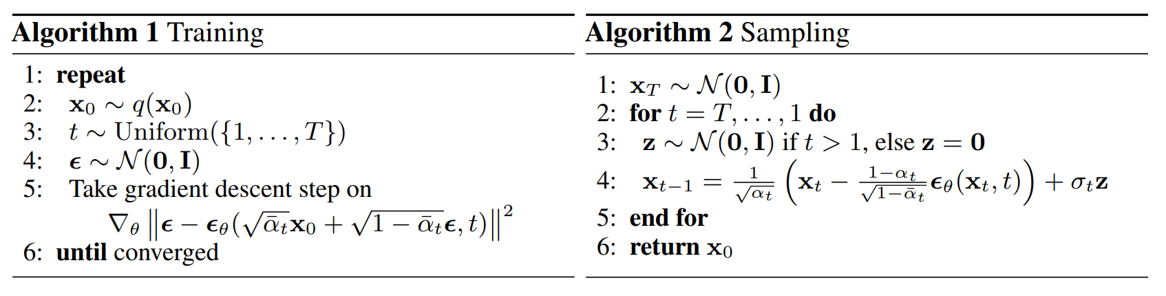
Let’s first look at the training algorithm:
- We repeat the below process (steps 2~5) until convergence or a preset number of epochs.
- Sample an image \(x_0\) from our dataset/data distribution, \(q(x_0)\).
- Sample t, or timestep from 1 to \(T\).
- Sample noise from a normal distribution \(\epsilon \sim \mathcal{N}(0, I)\)
- Take gradient descent step on the training objective we just derived \(L_{LDM} = ||\epsilon - \epsilon_{\theta}(x_t,t)||^2\) with respect to \(\theta\), which is the parameters of the weights and biases of the decoder.
Not too bad! What about the above sampling algorithm?
Before describing the sampling process, let’s look back at the training objective, specifically regarding the value of T, or the timesteps for the forward process. Above, we described this as a Markovian process, and ideally we would like to maximize \(T\) or the number of timesteps in the forward diffusion so that the reverse process can be as close to a Gaussian as possible so that the generative process is accurate and generates a good image quality.
However, in this Markovian sampling process called DDPM (short for Denoising Diffusion Probabilistic Models), the \(T\) timesteps have to be performed sequentially, meaning sampling speed is extremely slow, especially compared to fast sampling speeds of predecessors such as GANs. The limitation here is that the forward \(T\) steps and the reverse sampling \(T\) steps must be equal, as we are reversing the forward process for sampling. The above Markovian sampling algorithm is the DDPM sampling algorithm, which will be explained first, but then we will also mention a new, non-Markovian sampling process called DDIM (short for Denoising Diffusion Implicit Models) that is able to accelerate sampling speeds. Note that the authors of the LDM paper utilized DDIM because of this exact reason.
Remember that for sampling, we only need the trained decoder from above (no encoder). Therefore, we sample latent noise \(x_T\) from prior \(p(x_T)\), which is \(\epsilon \sim \mathcal{N}(0, I)\) and then run the series of \(T\) equally weighted autoencoders as mentioned before in a Markovian style. The equation shown in the sampling algorithm is essentially identical to equation #4 above, or:
$$ \mu_{\theta} = \frac{1}{\sqrt{\alpha_t}}x_t - \frac{\sqrt{1-\alpha_t}}{\sqrt{1-\hat{\alpha_t}}\sqrt{\alpha_t}}\hat{\epsilon}_{\theta}(x_t,t) $$
The equation in the sampling algorithm at step #4 above just has an additional noise term \(\sigma_tz\) since the reparametrization trick \(x = \mu + \sigma_tz\). Note that in sampling, assuming our training went well, we have our trained neural network \(\hat{\epsilon}_{\theta}(x_t,t)\) that predicts the noise \(\epsilon\) for given input image \(x_t\) (remember that this neural network in our LDM is our U-Net architecture with the (cross) attention layers that predicts the noise given our input image). Then, inputting a timestep \(t\) and original image \(x_t\) to the trained neural network gives us the predicted noise \(\epsilon\), and using that we can sample \(x_{t-1}\) until \(t=1\). When \(t=1\), we have our sampled output of \(x_0\).
Let’s summarize this sampling algorithm:
- First sample Gaussian noise \(x_T\) from normal distribution.
- Then, reverse the timesteps for the forward diffusion, and for each timestep, sample noise \(z\) from another independent normal distribution. Note that when \(t=1\), we don’t want to further add noise. Lastly, for each timestep, sample \(x_{t-1}\) according to above equation.
- Repeat step #2 for each timestep until \(t=1\), and the generated sample is the desired \(x_0\).
However, as discussed above, Denoising Diffusion Implicit Model (DDIM) uses a non-Markovian sampling process that makes the process much quicker. DDPMs use a sampling process that is essentially the reverse of the forward diffusion (\(T\) forward and backward timesteps), while DDIM uses \(S\) steps instead of \(T\) where \(S<T\), by using the fact that the forward diffusion process can be made non-Markovian and therefore the reverse sampling process can also be made non-Markovian. Therefore, the authors of the LDM paper use DDIM over DDPM.
Recall the forward diffusion process mentioned in the previous part of the blog: \(x_t = \mathcal{N}(x_t; \mu_t = \sqrt{1-\beta_t}x_{t-1},\Sigma_t = \beta_tI)\). This is essentially the forward process of DDPMs, which we can see that the process is Markovian, as \(x_t\) only depends on \(x_{t-1}\). However, in the previous part of the blog, we’ve already shown the forward process that can be made non-Markovian when we were deriving the training objective. Recall the Baye’s rule we used to derive the mean and variance of the approximate denoising step: \(q(x_{t-1}|x_t,x_0) = \frac{q(x_t|x_{t-1},x_0)q(x_{t-1}|x_0)}{q(x_t|x_0)}\). Note by rearranging the above equation for the forward diffusion step \(q(x_t|x_{t-1},x_0)\) we see that the forward step is no longer Markovian, and this is the forward step for DDIM: \(q(x_t|x_{t-1},x_0) = \frac{q(x_{t-1}|x_t,x_0)q(x_t|x_0)}{q(x_{t-1}|x_0)}\)
With this non-Markovian forward diffusion step, the DDIM sampling process is also no longer forced to have the same number of timesteps \(T\). But how do we derive the DDIM sampling process? To derive the DDIM sampling process, we utilize the reparametrization trick again, which we applied previously for forward diffusion. We can use \(x = \mu + \sigma * \epsilon\) to essentially alter our sampling process \(q(x_{t-1}|x_t,x_0)\) to be parametrized by another random variable, a desired standard deviation \(\sigma_t\) (square this for variance). The reparametrization is shown below:
$$\text{Recall equation #1:} \text{ } x_t = \sqrt{\hat{\alpha}_t}x_0 + \sqrt{1-\hat{\alpha}_t}{\epsilon}_0 $$ $$\text{The equation for} \text{ } x_{t-1} \text{ } \text{instead is:} \text{ } x_{t-1} = \sqrt{\hat{\alpha}_{t-1}}x_0 + \sqrt{1-\hat{\alpha}_{t-1}}{\epsilon}_{t-1} $$ $$\text{Add extra term} \text{ } \sigma_t \epsilon \text{ } \text{for reparametrization trick, where} \text{ } \sigma_t^{2} \text{ } \text{is the variance of our distribution.}$$ $$ x_{t-1} = \sqrt{\hat{\alpha}_{t-1}}x_0 + \sqrt{1-\hat{\alpha}_{t-1}-\sigma_t^{2}}\epsilon_t + \sigma_t \epsilon $$ $$\text{Since} \text{ } \epsilon_t = \frac{x_t - \sqrt{\hat{\alpha_t}}x_0}{\sqrt{1-\hat{\alpha_t}}}: \text{ } x_{t-1} = \sqrt{\hat{\alpha}_{t-1}}x_0 + \sqrt{1-\hat{\alpha}_{t-1}-\sigma_t^{2}}\frac{x_t - \sqrt{\hat{\alpha_t}}x_0}{\sqrt{1-\hat{\alpha_t}}} + \sigma_t \epsilon $$ $$\text{Therefore,} \text{ } q(x_{t-1}|x_t,x_0) = \mathcal{N}(x_{t-1};\mu_{t-1} = \sqrt{1-\hat{\alpha}_{t-1}-\sigma_t^{2}}\frac{x_t - \sqrt{\hat{\alpha_t}}x_0}{\sqrt{1-\hat{\alpha_t}}},\Sigma_{t-1}= \sigma_t^{2}I)) $$ $$\text{Recall equation #15 from last blog for variance formulation:} $$ $$q(x_{t-1} \mid x_t,x_0) \sim \mathcal{N}(x_{t-1}; \mu_t = \frac{\sqrt{\alpha_t}(1-\hat{\alpha}_{t-1})x_t + \sqrt{\hat{\alpha}_{t-1}}(1-\alpha_t)x_0}{1-\hat{\alpha_t}},\Sigma_t = \frac{(1-\alpha_t)(1-\hat{\alpha}_{t-1})}{(1-\hat{\alpha_t})}I)$$ $$\text{Then, also recall that} \text{ } \beta_t = 1-\alpha_t \text{ ,} \text{ } \text{therefore our new variance:}$$ $$\hat{\beta_t} = \sigma_t^{2} = \frac{1-\hat{\alpha}_{t-1}}{1-\hat{\alpha_t}} * \beta_t $$
Above shows the mean and the variance of the DDIM denoising step. With above result, we can now let \(\eta = \frac{1-\hat{\alpha}_{t-1}}{1-\hat{\alpha_t}}\) and now \(\sigma_t^{2} = \eta * \hat{\beta_t}\) where \(\eta\) can now be used to control the stochasticity/determinism of the sampling process. As one can see, if \(\eta = 0\), this means that the variance of the above denoising step becomes zero and therefore the sampling becomes deterministic. This means that given an input image, no matter how many different times you sampled, you would end up with similar images with the same high-level features! Therefore, this is why this process is called “denoising diffusion implicit model”, as like other implicit models like GANs, the sampling process is deterministic.
But our main point was that DDIM dramatically speeds up the sampling process. We’ve shown that the forward process is non-Markovian, but how do we show that the reverse process requires fewer steps as well? Recall the derived sampling process from above:
$$x_{t-1} = \sqrt{\hat{\alpha}_{t-1}}x_0 + \sqrt{1-\hat{\alpha}_{t-1}-\sigma_t^{2}}\frac{x_t - \sqrt{\hat{\alpha_t}}x_0}{\sqrt{1-\hat{\alpha_t}}} + \sigma_t \epsilon $$
We will now aim to parametrize this sampling process for \(x_{t-1}\) in terms of our trained model. Here, we can see that given \(x_t\), we first make a prediction of \(x_0\), and then use both to make the prediction for \(x_{t-1}\). Now, recall the previously mentioned forward process \(q(x_t|x_0) = \mathcal{N}(x_t; \mu_t = \sqrt{\hat{\alpha}_t}x_0,\Sigma_t = (1-\hat{\alpha}_t)I)\). With reparametrization trick, we already showed that this gives our forward process to find \(x_t\) given \(x_0\) and our Gaussian noise \(\epsilon\): \(x_t = \sqrt{\hat{\alpha}_t}x_0 + \sqrt{1-\hat{\alpha}_t}{\epsilon}\). Rearranging the equation for \(x_0\) gives: \(x_0 = \frac{x_t - \sqrt{1-\hat{\alpha}_t}{\epsilon}}{\sqrt{\hat{\alpha}_t}}\). Now, here’s the important part, where do we utilize our trained model if this is the generative process? Recall from above again that our trained model \(\hat{\epsilon}_{\theta}(x_t,t)\) predicts noise \(\epsilon\) given \(x_t\) and timestep \(t\). Therefore, we rewrite the equation for \(x_0\) as:
$$x_0 = \frac{x_t - \sqrt{1-\hat{\alpha}_t}\hat{\epsilon}_{\theta}(x_t,t)}{\sqrt{\hat{\alpha}_t}}$$
Therefore, when we plug in this equation for \(x_0\) in original sampling process equation, we get:
$$x_{t-1} = \sqrt{\hat{\alpha}_{t-1}}\frac{x_t - \sqrt{1-\hat{\alpha}_t}\hat{\epsilon}_{\theta}(x_t,t)}{\sqrt{\hat{\alpha}_t}} + \sqrt{1-\hat{\alpha}_{t-1}-\sigma_t^{2}}\frac{x_t - \sqrt{\hat{\alpha_t}}x_0}{\sqrt{1-\hat{\alpha_t}}} + \sigma_t \epsilon $$.
But recall that when we rearrange the same equation \(x_t = \sqrt{\hat{\alpha}_t}x_0 + \sqrt{1-\hat{\alpha}_t}{\epsilon}\) in terms of \(\epsilon\), we get \(\epsilon = \frac{x_t - \sqrt{\hat{\alpha_t}}x_0}{\sqrt{1-\hat{\alpha_t}}}\). Therefore, we replace that term above with our trained model as well, giving us the final equation for \(x_{t-1}\) for DDIM sampling:
$$x_{t-1} = \sqrt{\hat{\alpha}_{t-1}}\frac{x_t - \sqrt{1-\hat{\alpha}_t}\hat{\epsilon}_{\theta}(x_t,t)}{\sqrt{\hat{\alpha}_t}} + \sqrt{1-\hat{\alpha}_{t-1}-\sigma_t^{2}}\hat{\epsilon}_{\theta}(x_t,t) + \sigma_t \epsilon_t $$. $$\text{where: }q(x_{t-1} \mid x_t,x_0) \sim \mathcal{N}(x_{t-1}; \mu_t = \frac{\sqrt{\alpha_t}(1-\hat{\alpha}_{t-1})x_t + \sqrt{\hat{\alpha}_{t-1}}(1-\alpha_t)x_0}{1-\hat{\alpha_t}},\Sigma_t = \frac{(1-\alpha_t)(1-\hat{\alpha}_{t-1})}{(1-\hat{\alpha_t})}I)$$
The above equation is the final equation that allows us to sample \(x_{t-1}\) from given \(x_t\) using our trained model. Suppose the forward process is non-Markovian now, and instead of having all of the Markovian steps from \(x_{1:T}\), we have a subset of \(S\) timesteps \({x_{\tau 1},....x_{\tau S}}\) where \(\tau\) is simply increasing sequence of \(S\) timesteps. Look at the figure below:
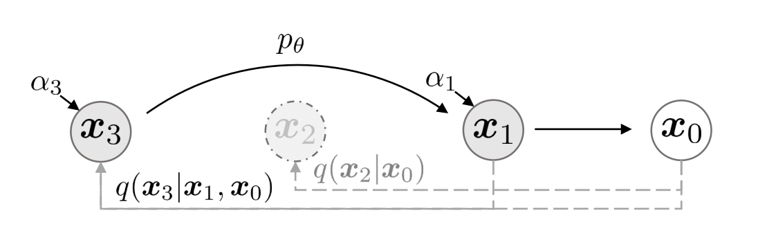
The diagram above is a simplified one in that \(\tau = [1,3]\), and the forward DDIM process \(q(x_3 \mid x_1,x_0)\) can be simply reversed by sampling using the above derived sampling process. Therefore, we see that DDIM utilizes a non-Markovian forward process that uses less timesteps which in turn allows it to use less computations in the reverse step as well.
$$x_{t-1} = \sqrt{\hat{\alpha}_{t-1}}\frac{x_t - \sqrt{1-\hat{\alpha}_t}\hat{\epsilon}_{\theta}(x_t,t)}{\sqrt{\hat{\alpha}_t}} + \sqrt{1-\hat{\alpha}_{t-1}-\sigma_t^{2}}\hat{\epsilon}_{\theta}(x_t,t) + \sigma_t \epsilon_t $$.
Now, let’s look back at each term of the right hand side of the above equation, the first term is the predicted \(x_0\) given \(x_t\). The second term can be interpreted as the direction pointing to \(x_t\), and the third term is random noise sampled from a normal distribution. With the above equation, we have two special cases depending on the value of \(\sigma_t\). First, when \(\sigma_t = \sqrt{\frac{1-\hat{\alpha}_{t-1}}{1-\hat{\alpha}_t}} \sqrt{\frac{1-\hat{\alpha}_t}{\hat{\alpha}_{t-1}}}\), the forward diffusion process actually becomes Markovian, which means that the sampling process naturally becomes DDPM as well. Second, like when \(\eta=0\) above, we see that when \(\sigma_t = 0\) for all timestep, we see that there is no stochasticity as there is no random noise added. With the exception for when \(t=1\), we see that the process is deterministic and therefore this is why samples generated are nearly identical or share the same high level features.
Lastly, another important note to make is that with the above equation, we can see that with the same trained model \(\hat{\epsilon}_{\theta}(x_t,t)\), we can have two different sampling methods DDPM and DDIM, with DDIM usually being superior over DDPM. Therefore, with DDIM, we do not need to retrain the model, which gives us another reason to use DDIM over DDPM.
To wrap up, the main advantages of DDIM over DDPM are:
- Faster sampling: As mentioned above, DDIM is a non-Markovian process that enables sample generation with a much smaller timestep \(S\), where \(S<T\) when \(T\) is the timestep required for DDPM. When the sampling trajectory \(S\) is much smaller than \(T\), we experience more computational efficiency at some cost of image generation quality.
- Control of stochasticity: As mentioned above, when \(\eta=0\) or \(\sigma_t=0\) for all timesteps, DDIMs are deterministic, meaning that if we start with the same latent vector (predicted noise) \(x_T\) via same random seed during sampling, the samples generated will all have the same high-level features.
- Allows interpolation: In DDPMs, interpolation is still possible, but the interpolation will not be accurate due to the stochasticity in the samples generated from DDPM. However, utilizing deterministic samples from DDIM allows us to not only generate our samples quickly, but also be able to interpolate between two different domains easily.
Therefore, we see that DDIM is a more efficient and effective sampling procedure over DDPM, and therefore, this is why the authors of the LDM paper use DDIM over DDPM. In the next and final part of the blog, we will cover conditioning and classifier/classifier-free guidance!
Image credits to: