(Concept Review/Generative Models) Latent/Stable Diffusion Fully Explained, Part 3
Table of Contents:
Latent/Stable Diffusion Fully Explained! (Part 1)
-
Introduction
-
Stable Diffusion vs GAN
Latent/Stable Diffusion Fully Explained! (Part 2)
-
Motivation
-
Model Architecture
-
Experiments & Results
Latent/Stable Diffusion Fully Explained! (Part 3) (This Blog!)
Latent/Stable Diffusion Fully Explained! (Part 4)
-
Different View on Model Objective
-
Training and Inference (DDIM vs DDPM)
Latent/Stable Diffusion Fully Explained! (Part 5- Coming Soon!)
-
Conditioning
-
Classifier-Free Guidance
-
Summary
Note: For other parts, please click the link above in the table of contents.
Stable Diffusion In Numbers
In this part of the blog, I will cover the mathematical details behind latent diffusion that is necessary to fully understand how latent diffusion works. This one took longer to write, as it is mathematically heavy, but it will be eventually worth it since understanding the underlying math will allow us to really fully understand stable diffusion. Before looking at the model objective of LDMs, I think it’s important to do an in-depth review on VAEs and how the Evidence Lower Bound (ELBO) is utilized:
VAEs and ELBO:
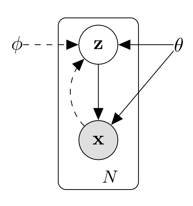
Let’s look at variational autoencoders (VAEs) in a probabilistic way. The variational autoencoder holds a probability model with the \(x\) representing the data, and the \(z\) representing the latent variables of the autoencoder. Remember that we want our latent variable \(z\) to model the data \(x\) as accurately as possible. Note that \(x\) can be seen, but \(z\) cannot since it is in the latent space. To perform the generative process, or run inference, for each individual data \(j\), we first sample latent variable \(z_i\) from the prior \(P(z)\): \(z_i \sim P(z)\). Then, with the prior sampled, we sample an individual data \(x_i\) from the likelihood \(P(x | z)\): \(x_i \sim P(x | z)\). Precisely, this can be represented in a graphical model below where we can see that the observed data \(x\) is conditioned on unobserved latent variable \(z\).
Now, remember again our goal in running inference in the VAE model is to model the latent space as good as possible given our data. This is Bayesian Inference, as “inference” means calculating the posterior probability, in this case the \(P(z | x)\). How do we calculate this? Let’s look at the classic Baye’s Rule:
$$P(z | x) = \frac{P(x | z)\cdot P(z)}{P(x)}$$
In this case, each variable is:
\(P(z)\) is the prior probability of \(z\), which is the initial belief without any knowledge about \(x\).
\(P(x)\) is the evidence, or the marginal likelihood, the probability of observing \(x\) across all possible events.
\(P(z | x)\) is the posterior probability of \(z\) given \(x\).
\(P(x | z)\) is the likelihood of observing \(x\) given \(z\), which assumes the prior is correct.
From above, let’s focus on the evidence, or the marginal likelihood. \(P(x)\) can be calculated by: \(P(x) = \displaystyle \int P(x | z)P(z) dz\) since we have a continuous distribution (in VAEs, the latent variable z is assumed to specified to be a Gaussian distribution with a mean of zero and unit variance (\(\mathcal{N}(0, 1)\)). However, this simple-looking integral over the product of gaussian conditional and prior distribution is intractable because the integration is performed over the entire latent space, which is continuous (it is possible to have infinite number of latent variables for a single input).
But can we try calculating \(P(x)\) in a different way? We also know that the joint probability \(P(x,z) = P(x)P(z | x)\), meaning that \(P(x) = \frac{P(x,z)}{P(z | x)}\). We quickly realize that this doesn’t work either since we already saw above that the posterior \(P(z | x)\) is unknown! Therefore, we have to resort to approximating the posterior \(P(z | x)\) with an approximate variational distribution \(q_\phi(z | x)\) which has parameters \(\phi\) that needs to be optimized. Hence, in the previous graphical model, the dashed arrow going from x to z represents the variational approximation.
But how do we ensure that our approximate variational distribution \(q_\phi(z | x)\) will be as similar as possible to the intractable posterior \(P(z | x)\)? We do this by minimizing the KL-divergence between the two distributions. For two distributions P and Q, KL-divergence essentially measures the difference between the two distributions. The value of the KL-divergence cannot be less than zero, as zero denotes that the two distributions are perfectly equal to each other. Note that \(D_{KL}(P || Q) = \sum_{n=i} P(i) \log \frac{P(i)}{Q(i)}\)
Now let’s expand on this:
$$min(D_{KL}(q(z|x) || P(z|x))) = - \sum_{n=i} q(z|x) \log \frac{P(z|x)}{q(z|x)}$$ $$min(D_{KL}(q(z|x) || P(z|x))) = - \sum_{n=i} q(z|x) \log \frac{P(x,z)}{q(z|x)P(x)} \quad \text{since} \ P(z|x) = \frac {P(x,z)}{P(x)}$$ $$min(D_{KL}(q(z|x) || P(z|x))) = - \sum_{n=i} q(z|x) [\log \frac{P(x,z)}{q(z|x)} - \log P(x)]$$ $$min(D_{KL}(q(z|x) || P(z|x))) = - \sum_{n=i} q(z|x) \log \frac{P(x,z)}{q(z|x)} + \sum_{n=i} q(z|x) \log P(x)$$ $$min(D_{KL}(q(z|x) || P(z|x))) = - \sum_{n=i} q(z|x) \log \frac{P(x,z)}{q(z|x)} + \log P(x) \quad \text{since} \ \sum_{n=i} q(z|x) = 1$$ $$\log P(x) = min(D_{KL}(q(z|x) || P(z|x))) + \sum_{n=i} q(z|x) \log \frac{P(x,z)}{q(z|x)} \quad (1)$$
Observe the left hand side of the last line above (or equation #1). Since we observe \(x\), this is simply a constant. Observe the right hand side now. The first term is what we initially wanted to minimize. The second term is what’s called an “evidence/variational lower bound”, or “ELBO” for short. This is because rather than minimizing our first term (KL-divergence), utilizing the fact that the KL-divergence is always greater than or equal to zero, we can rather maximize the ELBO instead. We know understand why the second term is called a “lower bound”, as \(ELBO \leq \log P(x)\) since \(D_{KL}(q(z|x) || P(z|x)) \geq 0\) all the time.
Now let’s expand on ELBO:
$$ ELBO = \sum_{n=i} q(z|x) \log \frac{P(x,z)}{q(z|x)}$$ $$ ELBO = \sum_{n=i} q(z|x) \log \frac{P(x|z)P(z)}{q(z|x)}$$ $$ ELBO = \sum_{n=i} q(z|x) [\log P(x|z) + \log \frac{P(z)}{q(z|x)}]$$ $$ ELBO = \sum_{n=i} q(z|x) \log P(x|z) + \sum_{n=i} q(z|x) \log \frac{P(z)}{q(z|x)}$$ $$ ELBO = \sum_{n=i} q(z|x) \log P(x|z) - D_{KL}(q(z|x) || P(z))$$ $$ ELBO = \mathbb{E}_{q(z|x)} [\log P(x|z)] - D_{KL}(q(z|x) || P(z)) \quad (2)$$
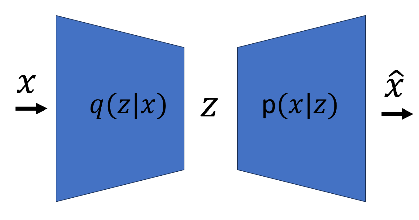
Remember the last line above (or equation #2) for later, this is also the loss function for training VAEs. But to understand this expression better, let’s now look at VAEs in a neural network’s perspective. A VAE consists of an encoder and a decoder, and both are neural networks. The encoder takes in input data \(x\) and compresses it to latent representation \(z\), and must learn a good latent representation known as the bottleneck of the model. Note that contrary to the encoder of the vanilla autoencoder, the encoder of the variational autoencoder will learn the mean and variance Therefore, the encoder can be denoted as \(q_\phi(z | x)\), where the \(\phi\) is the weights and biases of the model. Note that as previously mentioned, the latent space is assumed to be a Gaussian probability distribution, so sampling from the trained encoder gets us the latent representation \(z\) from data \(x\). The decoder takes in the latent representation z from the encoder output and outputs the reconstructed data denoted as \(\hat{x}\), or the parameters to the modeled probability distribution of the data space, and therefore can be denoted as \(p_\theta(x | z)\), where \(\theta\) is also the weights and biases. The below diagram helps us see this entire scheme.
Now let’s go back to above equation #2. Let’s look at the first term \(\mathbb{E}_{q(z|x)} [\log P(x|z)]\). Now, remember that the latent space \(z\) is assumed to be a Gaussian distribution \(z_i \sim \mathcal{N}(0,1)\). Observe this:
$$\log p(x|z) \sim \log exp(-(x-f(z))^2$$ $$\sim |x-f(z)|^2 $$ $$ = |x-\hat{x}|^2 $$
where \(f(z) = \hat{x}\), as the reconstructed image \(\hat{x}\) is the distribution mean \(f(z)\). This is because \(p(x|z) \sim \mathcal{N}(f(z), I)\). Therefore, here we see that the first term is correlated to the mean squared error (MSE) loss between the original image and the reconstructed image. This makes sense, as during training, we want to make penalize the model if the reconstructed image is too dissimilar to the original image. It is important to see that this was the first term of the ELBO, and remember we want to maximize this. Maximizing the first term is then therefore correlated to minimizing the MSE/reconstruction loss.
Let’s now look at the second term, \(-D_{KL}(q(z|x) || P(z))\) (note the negative sign) which is the KL-divergence between our learned gaussian distribution (encoder) \(q(z|x)\) and the prior (latent space) gaussian distribution. Remember this is the second term of ELBO, so we still want to maximize- but note the negative sign, we actually want to minimize the KL divergence between the two- which makes sense as we want to encourage the learned distribution from the encoder to be similar to the unit Gaussian prior.
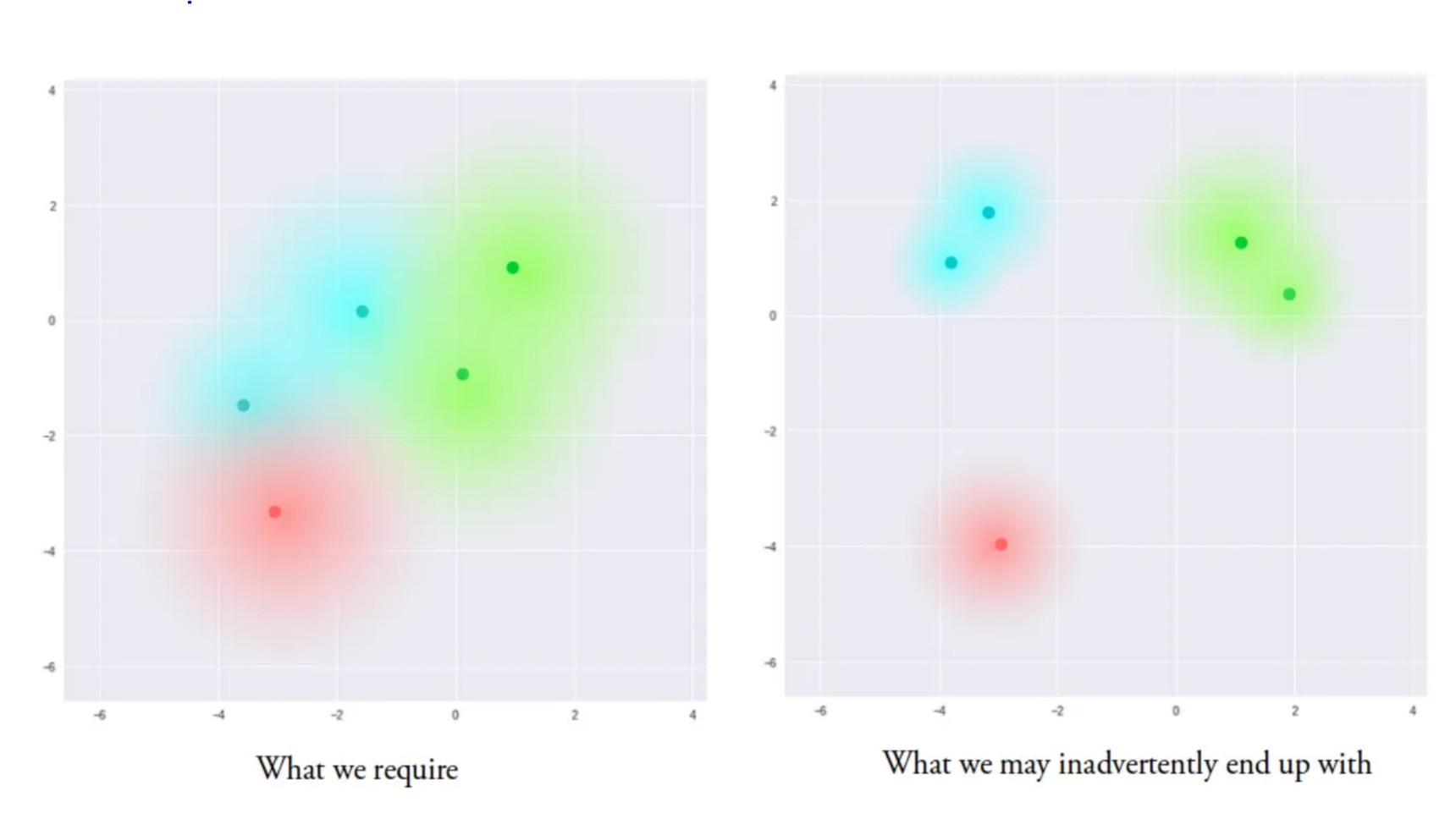
This actually ties back to the KL-regularization of LDMs in the previous blog (part 2), which is the diagram showing the VAE latent space with and without KL-regularization. This is re-shown above. The minimization of KL divergence shown above regularizes the latent space as the “clusters” itself are bigger and are more centered around within each other. This ensures that the decoder creates diverse and accurate samples, as there would be smoother transitions between different classes (clusters). This is why both reconstruction loss term and KL-divergence term are included in the VAE loss function during training.
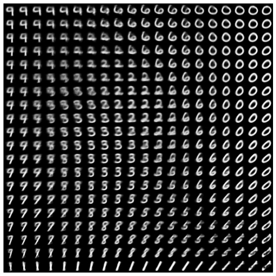
For example, as seen above for MNIST handwritten digits, we see that the classes, or clusters have a smooth transition in this latent space. Without regularization, the encoder can cheat by learning narrow distributions with low variances. Now that we’ve understood the importance of maximizing ELBO to train a VAE, let’s go back to LDMs.
Model Objective:
Now why did we go over the VAEs and its variational approximation process? This is because diffusion models have a very similar set up to VAEs in that it also has a tractable likelihood that can be maximized by maximizing the ELBO to ensure that the approximate posterior is as similar as possible to the unknown true posterior we’d like to model. We’re going to derive the training loss function, or the model objective just like how it was done for VAEs.
Let’s first look at the forward and the backward diffusion process in a probabilistic way, since we already know about the diffusion processes in neural networks (train a regularized autoencoder for forward and backward diffusion process!). Take a look at the graphical model below:
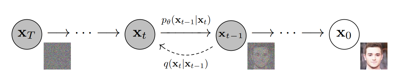
The forward diffusion process actually is the reverse of the above diagram, as the arrows should be going the opposite way- the forward diffusion process adds noise to a specific data point \(x_0\) that is sampled from the unknown, true distribution we’d like to model. Then, \(x_0\) has Gaussian noise added to it in a Markovian process (from \(x_{t-1}\) all the way to \(x_T\)) with \(T\) steps. Therefore, \(q(x_t|x_{t-1})\) takes the image and outputs a slightly more noisy version of the image. This can be formulated below:
$$q(x_t|x_{t-1}) = \mathcal{N}(x_t; \mu_t = \sqrt{1-\beta_t}x_{t-1},\Sigma_t = \beta_tI) \quad (3)$$
Assuming high-dimensionality, \(q(x_t|x_{t-1})\) is a Gaussian distribution with the above defined mean and variance. Note that for each dimension, it has the same variance \(\beta_t\). \(\beta_t\) is a number between 0 and 1, and essentially scales the data so the variance doesn’t grow out of proportion. The authors use a linear schedule for \(\beta_t\), meaning that \(\beta_t\) is linearly increased as the image gets noised more. Note that with above formula, we can easily obtain desired noised image at timestep \(T\) by using the Markovian nature of the process. Below is a tractable, closed-form formula to sample a noised image at any timestep:
$$q(x_{1:T}|x_0) = \prod_{t=1}^{T} q(x_t|x_{t-1}) \quad (4)$$
Basically, if T = 200 timesteps, we would have 200 products to sample the noised image \(x_{t=200}\). However, if the timestep gets larger, we run in to trouble of computational issues. Therefore, we utilize the reparametrization trick which gives us a much simpler tractable, closed-form formula for sampling that requires much fewer computations.
The reparametrization trick is used whenever we sample from a distribution (Gaussian in our case) that is not directly differentiable. For our case, the mean and the variance of the distribution are both dependent on the model parameters, which is learned through SGD (as shown above). The issue is that because sampling from the Gaussian distribution is stochastic, we cannot compute the gradient anymore to update the mean and variance parameters. So, we introduce the auxiliary random variable \(\epsilon\) that is deterministic since it is sampled from a fixed standard Gaussian distribution (\(\epsilon \sim \mathcal{N}(0, 1)\)), which allows SGD to be possible since \(\epsilon\) is not dependent on the model parameters. Therefore, the reparametrization trick \(x = \mu + \sigma * \epsilon\) works by initially computing the mean and standard deviation using current weights given input data, then drawing deterministic random variable \(\epsilon\) to obtain the desired sample \(x\). Then, loss can be computed with respect to mean and variance, and they can be backpropagated via SGD.
$$ \text{Let} \quad \alpha_t = 1 - \beta_t \text{and} \quad \hat{\alpha}_t = \prod_{i=1}^{t} \alpha_i $$ $$ \text{Also sample noise} \quad \epsilon_0, ..., \epsilon_{t-1} \sim \mathcal{N}(0,I) $$ $$ \text{Then,} \quad x_t = \sqrt{1-\beta_t}x_{t-1} + \sqrt{\beta_t}\epsilon_{t-1} $$ $$ x_t = \sqrt{\alpha_t}x_{t-1} + \sqrt{1-\alpha_t}\epsilon_{t-1} $$ $$ x_t = \sqrt{\alpha_t \alpha_{t-1}}x_{t-2} + \sqrt{1-\alpha_t \alpha_{t-1}}\epsilon_{t-2} $$ $$ x_t = \quad ... $$ $$ x_t = \sqrt{\hat{\alpha}_t}x_0 + \sqrt{1-\hat{\alpha}_t}{\epsilon}_0 $$ $$ \mathbf{ \text{Therefore, since } \quad \mu + \sigma * \epsilon, \quad q(x_t|x_0) = \mathcal{N}(x_t; \mu_t = \sqrt{\hat{\alpha}_t}x_0,\Sigma_t = (1-\hat{\alpha}_t)I)} \quad (5)$$
Note that above simplification is possible since the variance of two merged Gaussians is simply the sum of the two variances.
To summarize the forward diffusion process, we can think of this as the encoder (remember encoder performs forward diffusion process to map pixel space to latent space) Each time step or each encoder transition is denoted as \(q(x_t|x_{t-1})\) which is from a fixed parameter \(\mathcal{N}(x_t,\sqrt{\alpha_t}x_{t-1},(1-\alpha_t)I)\). Note that like VAE encoder, the encoder distribution for the forward diffusion process is also modeled as multivariate Gaussian. However, in VAEs, we learn the mean and variance parameters, while forward diffusion has fixed specific means and variances at each timestep as seen in equation #4.
Now, look at the graphical model again for the reverse diffusion process, which is denoted by \(p_\theta(x_{t-1}|x_t)\). Now, if we could reverse the above forward diffusion process \(q(x_t|x_{t-1})\) and sample from \(q(x_{t-1}|x_t)\), we can easily run inference by sampling from our Gaussian noise input which is \(\sim \mathcal{N}(0,I)\). However, this is exactly the same problem we had for VAEs as above ! This true posterior is unknown and is intractable since we have to compute the entire data distribution or marginal likelihood/evidence, \(q(x)\). Here, we can treat \(x_0\) as the true data, and every subsequent node in the Markovian chain \(x_1,x_2...x_T\) as a latent variable. Therefore, we approach this problem the exact same way.
We approximate the true posterior \(q(x_{t-1}|x_t)\) with a neural network or a “decoder” that has parameters \(\theta\) (Note that this denoising diffusion “decoder” is the UNet, please don’t confuse this to the decoder of the autoencoder, which is something completely different as it is responsible for bringing the final output of \(x_0\) back to the pixel space. As previously discussed, we utilize UNet because of its inductive bias to images and its compatibility with cross attention). Like the forward process, but just reversing the timestep, we have:
$$ p_{\theta}(x_{0:T}) = p(x_T) \prod_{t=1}^{T} p_{\theta}(x_{t-1}|x_t) = \mathcal{N}(x_{t-1}; \mu_{\theta}(x_t,t),\Sigma_{\theta}(x_t,t)) \quad (6)$$
This is just like the forward process in equation #4 but in reverse. By applying this formula, we can go from pure noise \(x_T\) to the approximated data distribution. Remember the encoder does not have learnable parameters (pre-defined or fixed), so we only need to train the decoder in learning the conditionals \(p_{\theta}(x_{t-1}|x_t)\) so we can generate new data. Conditioning on the previous timestep \(t\) and previous latent \(x_t\) lets the decoder learn the Gaussian parameters \(\theta\) which is the mean and variance \(\mu_{\theta},\Sigma_{\theta}\) (Since we assume variance is fixed due to noise schedule \(\beta\), however, we just need to learn the mean with the decoder). Therefore, running inference on a LDM only requires the decoder as we sample from pure Gaussian noise \(p(x_T)\) and run T timesteps of the decoder transition \(p_{\theta}(x_{t-1}|x_t)\) to generate new data sample \(x_0\). If our approximated \(p_{\theta}(x_{t-1}|x_t)\) steps are similar to unknown, true posterior steps \(q(x_{t-1}|x_t)\), the generated sample \(x_0\) will be similar to the one sampled from the training data distribution.
Therefore, we want to train our decoder to find the reverse Markov transitions that will maximize the likelihood of the training data. Now, how do we train this denoising/reverse diffusion model? We utilize the ELBO again. Remember for equation #1, we saw that the VAE was optimized by maximizing the ELBO (which was essentially the same as minimizing the negative log likelihood), we do the same below. Like VAEs, we first want to minimize the KL-divergence between the true unknown posterior \(q(x_{1:T}|x_0)\) and the approximated posterior \(p_{\theta}(x_{1:T}|x_0)\):
$$ 0 \leq min \ D_{KL}(q(x_{1:T}|x_0)||p_{\theta}(x_{1:T}|x_0)) $$ $$ - \log (p_{\theta}(x_0)) \leq - \log (p_{\theta}(x_0)) + min \ D_{KL}(q(x_{1:T}|x_0)||p_{\theta}(x_{1:T}|x_0)) $$ $$ - \log (p_{\theta}(x_0)) \leq - \log (p_{\theta}(x_0)) + \log(\frac{q(x_{1:T}|x_0)}{p_{\theta}(x_{1:T}|x_0)})$$ $$ - \log (p_{\theta}(x_0)) \leq - \log (p_{\theta}(x_0)) + \log(\frac{q(x_{1:T}|x_0)}{p_{\theta}(x_{0:T})}) + \log(p_{\theta}(x_0)) \quad \text{since} \ p_{\theta}(x_{1:T}|x_0) = \frac{p_{\theta}(x_0|x_{1:T})p_{\theta}(x_{1:T})}{p_{\theta}(x_0)} = \frac{p_{\theta}(x_0,x_{1:T})}{p_{\theta}(x_0)} = \frac{p_{\theta}(x_{0:T})}{p_{\theta}(x_0)}$$ $$ - \log (p_{\theta}(x_0)) \leq \log(\frac{q(x_{1:T}|x_0)}{p_{\theta}(x_{0:T})}) \quad \text{since} \ - \log (p_{\theta}(x_0)) + \log(p_{\theta}(x_0)) = 0 \quad (7)$$
As seen in above, minimizing the KL-divergence also gives us the form \(- \log P(x) \leq ELBO\) or \(-ELBO \leq \log P(x)\), as we saw for VAEs in equation #1, since the RHS of equation #7 above is the ELBO for LDMs (\(ELBO_{LDM} = \log(\frac{q(x_{1:T}|x_0)}{p_{\theta}(x_{0:T}})\)). Therefore, instead of minimizing the above KL-divergence, we can maximize the ELBO like VAEs:
$$ - \log (p_{\theta}(x_0)) \leq \log(\frac{q(x_{1:T}|x_0)}{p_{\theta}(x_{0:T})}) $$ $$ - \log (p_{\theta}(x_0)) \leq \log(\frac{\prod_{t=1}^{T} q(x_t|x_{t-1})}{p(x_T) \prod_{t=1}^{T}p_{\theta}(x_{t-1}|x_t)}) \quad \text{since} \ p_{\theta}(x_{0:T}) = p(x_T) \prod_{t=1}^{T} p_{\theta}(x_{t-1}|x_t)$$ $$ - \log (p_{\theta}(x_0)) \leq - \log(p(x_T)) + \log (\frac{\prod_{t=1}^{T} q(x_t|x_{t-1})}{\prod_{t=1}^{T}p_{\theta}(x_{t-1}|x_t)}) $$ $$ - \log (p_{\theta}(x_0)) \leq - \log(p(x_T)) + \sum_{t=1}^{T} \log(\frac{q(x_t|x_{t-1})}{p_{\theta}(x_{t-1}|x_t)}) $$ $$ - \log (p_{\theta}(x_0)) \leq - \log(p(x_T)) + \sum_{t=2}^{T} \log(\frac{q(x_t|x_{t-1})}{p_{\theta}(x_{t-1}|x_t)}) + \log(\frac{q(x_1|x_0)}{p_{\theta}(x_0|x_1)}) \quad \text{since} \ \log(\frac{q(x_1|x_0)}{p_{\theta}(x_0|x_1)}) \ \text{is when} \ t = 1 \quad (8)$$
Note equation #8 above, and focus on \(q(x_t|x_{t-1})\) term. This is essentially the reverse diffusion step, but it is only conditioned on the pure Gaussian noise. The latent image vector \(x_{t-1}\) thus has a high variance, but by also conditioning on original image \(x_0\), we can decrease the variance and therefore enhance the image generation quality (think about it, if model is conditioned only on pure Gaussian noise, the produced latent image would vary more than the model conditioned on pure Gaussian noise and the original image as well). This is achieved by using the Baye’s rule:
$$q(x_t|x_{t-1}) = \frac{q(x_{t-1}|x_t)q(x_t)}{q(x_{t-1})} = \frac{q(x_{t-1}|x_t,x_0)q(x_t|x_0)}{q(x_{t-1}|x_0)}$$
Substituting this to equation #8 gives equation #9:
$$ - \log (p_{\theta}(x_0)) \leq - \log(p(x_T)) + \sum_{t=2}^{T} \log(\frac{q(x_{t-1}|x_t,x_0)q(x_t|x_0)}{p_{\theta}(x_{t-1}|x_t)q(x_{t-1}|x_0)}) + \log(\frac{q(x_1|x_0)}{p_{\theta}(x_0|x_1)}) \quad (9)$$
For equation #9, we can further split the second term on the RHS (the summation term) to two different summation terms to further simplify the RHS:
$$ \sum_{t=2}^{T} \log(\frac{q(x_{t-1}|x_t,x_0)q(x_t|x_0)}{p_{\theta}(x_{t-1}|x_t)q(x_{t-1}|x_0)}) = \sum_{t=2}^{T} \log(\frac{q(x_{t-1}|x_t,x_0)}{p_{\theta}(x_{t-1}|x_t)}) + \sum_{t=2}^{T} \log(\frac{q(x_t|x_0)}{q(x_{t-1}|x_0)})$$
Examining \(\sum_{t=2}^{T} \log(\frac{q(x_t|x_0)}{q(x_{t-1}|x_0)})\), for any \(t>2\), we see that all the terms in the denominator and numerator will cancel out each other and will simplify to \(\log(\frac{q(x_t|x_0)}{q(x_1|x_0)})\).
Performing all of these substitutions to equation #9 gives equation #10:
$$- \log (p_{\theta}(x_0)) \leq - \log(p(x_T)) + \sum_{t=2}^{T} \log(\frac{q(x_{t-1}|x_t,x_0)}{p_{\theta}(x_{t-1}|x_t)}) + \log(\frac{q(x_t|x_0)}{q(x_1|x_0)}) + \log(\frac{q(x_1|x_0)}{p_{\theta}(x_0|x_1)}) \quad (10)$$
Now take the last two terms of the RHS in equation #10 above and further simplify by expanding the log:
$$- \log (p_{\theta}(x_0)) \leq - \log(p(x_T)) + \sum_{t=2}^{T} \log(\frac{q(x_{t-1}|x_t,x_0)}{p_{\theta}(x_{t-1}|x_t)}) + \log(q(x_t|x_0)) - \log(q(x_1|x_0)) + \log(q(x_1|x_0)) - \log(p_{\theta}(x_0|x_1))$$ $$- \log (p_{\theta}(x_0)) \leq - \log(p(x_T)) + \sum_{t=2}^{T} \log(\frac{q(x_{t-1}|x_t,x_0)}{p_{\theta}(x_{t-1}|x_t)}) + \log(q(x_t|x_0)) - \log(p_{\theta}(x_0|x_1))$$ $$- \log (p_{\theta}(x_0)) \leq \log(\frac{q(x_t|x_0)}{p(x_T)}) + \sum_{t=2}^{T} \log(\frac{q(x_{t-1}|x_t,x_0)}{p_{\theta}(x_{t-1}|x_t)}) - \log(p_{\theta}(x_0|x_1))$$ $$- \log (p_{\theta}(x_0)) \leq D_{KL}(q(x_T|x_0)||p(x_T)) + \sum_{t=2}^{T} D_{KL}(q(x_{t-1}|x_t,x_0)||p_{\theta}(x_{t-1}|x_t)) - \log(p_{\theta}(x_0|x_1)) \quad (11)$$
Now look at equation #11 above, which is simplified further thanks to the definition of KL-divergence. The first RHS term \(D_{KL}(q(x_T|x_0)||p(x_T))\) has no learnable parameters, as we previously talked about the encoder \(q(x_T|x_0)\) having no learnable parameters as the forward diffusion process is fixed by the noising schedule shown in equation #3 and #5. Additionally, \(p(x_T)\) is just pure Gaussian noise as well. Lastly, it is safe to assume that this term will be zero, as q will resemble p’s random Gaussian noise and bring the KL-divergence to zero. Therefore, below is our final training objective, all we need to do is minimize the RHS of the equation:
$$ - \log (p_{\theta}(x_0)) \leq \sum_{t=2}^{T} D_{KL}(q(x_{t-1}|x_t,x_0)||p_{\theta}(x_{t-1}|x_t)) - \log(p_{\theta}(x_0|x_1)) \quad (12)$$
Now, to minimize the RHS of the equation our only choice is to minimize the first term \(\sum_{t=2}^{T} D_{KL}(q(x_{t-1}|x_t,x_0)||p_{\theta}(x_{t-1}|x_t))\). Before diving into the derivation, let’s look at what this term actually means- it is the KL divergence between the ground truth denoising transition step \(q(x_{t-1}|x_t,x_0)\) and our approximation of the denoising transition step \(p_{\theta}(x_{t-1}|x_t)\), and it makes sense we want to minimize this KL divergence since we want the approximated denoising transition step to be as similar to the ground truth denoising transition step as possible.
Utilizing Baye’s Rule, we can calculate the desired ground truth denoising step \(q(x_{t-1}|x_t,x_0)\) :
$$ q(x_{t-1}|x_t,x_0) = \frac{q(x_t|x_{t-1},x_0)q(x_{t-1}|x_0)}{q(x_t|x_0)} \quad (13) $$
Now, we know the form of the distribution of the denominator of equation #13 above, which is \(q(x_t|x_0) = \mathcal{N}(x_t; \mu_t = \sqrt{\hat{\alpha_t}}x_0,\Sigma_t = (1-\hat{\alpha_t})I)\) Recall that this is from equation #5 from above and this was the reparametrization trick for the simplification of the forward diffusion process, or \(q(x_t|x_0)\) : \(x_t = \sqrt{\hat{\alpha}_t}x_0 + \sqrt{1-\hat{\alpha}_t}\epsilon\).
Now, how about the numerator? We also know the forms of the two distributions in the numerator of equation #1 above as well. \(q(x_t \mid x_{t-1},x_0)\)is the forward diffusion noising step and is formulated in equation #3 above \(q(x_t \mid x_{t-1}) = \mathcal{N}(x_t; \mu_t = \sqrt{1-\beta_t}x_{t-1},\Sigma_t = \beta_tI) = q(x_t \mid x_{t-1}, x_0) = \mathcal{N}(x_t; \mu_t = \sqrt{\alpha_t}x_{t-1},\Sigma_t = (1-\alpha_t)I)\) where \(\alpha_t = 1-\beta_t\). The other distribution \(q(x_{t-1} \mid x_0)\) is a slight modification of the distribution in the numerator \(q(x_t|x_0)\), with \(t\) being \(t-1\) instead, so this is formulated as:
$$q(x_{t-1} \mid x_0) = \mathcal{N}(x_{t-1}; \mu_t = \sqrt{\hat{\alpha}_{t-1}}x_0,\Sigma_t = (1-\hat{\alpha}_{t-1})I)$$
Now inputting all three of these formulations in the Baye’s Rule above in equation #13 we get equation #14 below:
$$q(x_{t-1} \mid x_t,x_0) = \frac{\mathcal{N}(x_t; \mu_t = \sqrt{\alpha_t}x_{t-1},\Sigma_t = (1-\alpha_t)I) \mathcal{N}(x_{t-1}; \mu_t = \sqrt{\hat{\alpha}_{t-1}}x_0,\Sigma_t = (1-\hat{\alpha}_{t-1})I)}{\mathcal{N}(x_t; \mu_t = \sqrt{\hat{\alpha}_t}x_0,\Sigma_t = (1-\hat{\alpha}_t)I)} \quad (14)$$
Now, combining the three different Gaussian distributions above to get the mean and variance for the desired \(q(x_{t-1} \mid x_t,x_0)\) is a lot of computations to show in this blog. The full derivation, for those who are curious, can be found in this link, exactly in page 12 from equation 71 to 84. (I just feel like this derivation is just a bunch of reshuffling variables with algebra, so it is unnecessary to include in my blog) Finishing this derivation shows that our desired \(q(x_{t-1} \mid x_t,x_0)\) is also normally distributed with the below formulation:
$$q(x_{t-1} \mid x_t,x_0) \sim \mathcal{N}(x_{t-1}; \mu_t = \frac{\sqrt{\alpha_t}(1-\hat{\alpha}_{t-1})x_t + \sqrt{\hat{\alpha}_{t-1}}(1-\alpha_t)x_0}{1-\hat{\alpha_t}},\Sigma_t = \frac{(1-\alpha_t)(1-\hat{\alpha}_{t-1})}{(1-\hat{\alpha_t})}I \quad (15)$$
From above, we can see that the above approximate denoising transition \(q(x_{t-1} \mid x_t,x_0)\) has mean that is a function of \(x_t\) and \(x_0\) and therefore can be abbreviated as \(\mu_q(x_t,x_0)\), and has variance that is a function of \(t\) (naturally) and the \(\alpha\) coefficients and therefore can be abbreviated as \(\Sigma_q(t)\). Recall that these \(\alpha\) coefficients are fixed and known, so that at any time step \(t\), we know the variance.
Now, back to equation #12 where we want to minimize the KL-divergence:
$$ \mathop{\arg \min}\limits_{\theta} \quad D_{KL}(q(x_{t-1} \mid x_t,x_0)||p_{\theta}(x_{t-1} \mid x_t)) $$
Equation #15 above tells us the formulation for ground truth denoising transition step \(q(x_{t-1} \mid x_t,x_0)\) , and we know the formulation for our approximate denoising transition step \(p_{\theta}(x_{t-1} \mid x_t)\).
What is the KL-divergence between two Gaussian distributions? It is:
$$ D_{KL}(\mathcal{N}(x;\mu_x,\Sigma_x) || \mathcal{N}(y;\mu_y,\Sigma_y)) = \frac{1}{2} [ \log \frac{\Sigma_y}{\Sigma_x} - d + tr({\Sigma_y}^{-1}\Sigma_x) + (\mu_y - \mu_x) ^ {T} {\Sigma_y}^{-1} (\mu_y - \mu_x) ] $$
Applying this KL-divergence equation to equation #12 above is also just reshuffling algebra, which is shown in the same link as before, from equations 87 to 92. We can see that equation #12 is simplified to:
$$ \mathop{\arg \min}\limits_{\theta} \quad \frac{1}{2{\sigma_q}^{2}(t)} [{|| \mu_{\theta} - \mu_q ||}^{2}] \quad (16) $$
To explain equation #16 above, \(\mu_q\) is the mean of the ground truth denoising transition step \(q(x_{t-1} \mid x_t,x_0)\) and \(\mu_{\theta}\) is the mean of our desired approximate denoising transition step \(p_{\theta}(x_{t-1} \mid x_t)\). How do we get these two values? We calculated them at equation 15, we can just utilize the \(\mu_t\), it depends on \(x_0\) and \(x_t\)! But wait, while \(q(x_{t-1} \mid x_t,x_0)\) is dependent on \(x_0\) and \(x_t\), \(p_{\theta}(x_{t-1} \mid x_t)\) is only dependent on \(x_t\), but not \(x_0\)! Well this is exactly what we’re trying to do, our approximate denoising step \(\hat{x}_{\theta}(x_t,t)\) is parametrized by the neural network with \(\theta\) parameters, we predict the generated/original image \(x_0\) using noisy image \(x_t\) and time step \(t\)!
We see why it’s important to do derivations, it exactly shows what the objective is here now: train a neural network that parametrizes \(\hat{x}_{\theta}(x_t,t)\) to predict \(x_0\) as accurately as possible to make our approximate denoising step as similar to the ground truth denoising step as possible! \(\mu_q\) and \(\mu_{\theta}\), using equation #15 is:
$$\mu_q = \frac{\sqrt{\alpha_t}(1-\hat{\alpha}_{t-1})x_t + \sqrt{\hat{\alpha}_{t-1}}(1-\alpha_t)x_0}{1-\hat{\alpha_t}}$$ $$\mu_{\theta} = \frac{\sqrt{\alpha_t}(1-\hat{\alpha}_{t-1})x_t + \sqrt{\hat{\alpha}_{t-1}}(1-\alpha_t)\hat{x}_{\theta}(x_t,t)}{1-\hat{\alpha_t}}$$
Note that the two are exactly the same except \(x_0\) is replaced with \(\hat{x}_{\theta}(x_t,t)\) as mentioned before. Finally, plugging these two into equation #16 allows us to find the training objective:
$$\mathop{\arg \min}\limits_{\theta} \quad \frac{1}{2{\sigma_q}^{2}(t)} [{ || \mu_{\theta} - \mu_q ||}^{2}] \quad $$ $$\mathop{\arg \min}\limits_{\theta} \quad \frac{1}{2{\sigma_q}^{2}(t)} [{ || \frac{\sqrt{\alpha_t}(1-\hat{\alpha}_{t-1})x_t + \sqrt{\hat{\alpha}_{t-1}}(1-\alpha_t)\hat{x}_{\theta}(x_t,t)}{1-\hat{\alpha_t}} - \frac{\sqrt{\alpha_t}(1-\hat{\alpha}_{t-1})x_t + \sqrt{\hat{\alpha}_{t-1}}(1-\alpha_t)x_0}{1-\hat{\alpha_t}} ||}^{2}]$$ The first term of each term is the same, so after eliminating those: $$\mathop{\arg \min}\limits_{\theta} \quad \frac{1}{2{\sigma_q}^{2}(t)} [{ || \frac{\sqrt{\hat{\alpha}_{t-1}}(1-\alpha_t)\hat{x}_{\theta}(x_t,t)}{1-\hat{\alpha_t}} - \frac{\sqrt{\hat{\alpha}_{t-1}}(1-\alpha_t)x_0}{1-\hat{\alpha_t}} ||}^{2}]$$ $$\mathop{\arg \min}\limits_{\theta} \quad \frac{1}{2{\sigma_q}^{2}(t)} [{ || \frac{\sqrt{\hat{\alpha}_{t-1}}(1-\alpha_t)}{1-\hat{\alpha_t}}(\hat{x}_{\theta}(x_t,t)-x_0)||}^{2}]$$ $$\mathop{\arg \min}\limits_{\theta} \quad \frac{1}{2{\sigma_q}^{2}(t)} \frac{\hat{\alpha}_{t-1}(1-\alpha_t)^{2}}{(1-\hat{\alpha_t)^{2}}} [{||(\hat{x}_{\theta}(x_t,t)-x_0)||}^{2}] \quad (17)$$
Equation #17 is finally our training objective. To summarize again, we are learning the parameters \({\theta}\) from training a neural network to predict the ground truth image \(x_0\) from noised version of the image \(x_t\). What’s important to take away from this, however, is understanding that, ultimately, applying the same ELBO method to maximize ELBO led to minimizing the KL divergence between ground truth and approximate denoising transition step, and this happens to be a form of minimizing the mean-squared-error (MSE) between the two distributions as seen in equation #17 above. This is quite fascinating, as all of this derivation just boils down to a simple MSE-like loss function.
Now, with the training objective derived, the training algorithms and sampling algorithms will be explained in the next two parts of this blog with more mathematical details on LDMs that were not covered yet, especially regarding training/inference algorithms and conditioning/classifier-free guidance.
Image credits to: