(Concept Review/Generative Models) Latent/Stable Diffusion Fully Explained, Part 2

Table of Contents:

Latent/Stable Diffusion Fully Explained! (Part 1)

• Introduction

• Why ditch GANs for Stable Diffusion?

Latent/Stable Diffusion Fully Explained! (Part 2) (This Blog!)

• Motivation

• Model Architecture

• Experiments & Results

Latent/Stable Diffusion Fully Explained! (Part 3)

• VAEs and ELBO

• Model Objective

Latent/Stable Diffusion Fully Explained! (Part 4)

• Different View on Model Objective

• Training and Inference (DDIM vs DDPM)

Latent/Stable Diffusion Fully Explained! (Part 5- Coming Soon!)

• Conditioning

• Classifier-Free Guidance

• Summary

Note: For other parts, please click the link above in the table of contents.

Stable Diffusion In Words:

In part 1, I’ve introduced the concept of generative models and the disadvantages of GANs, but that’s not all the motivation of the authors of the paper. Let’s first look at the author’s motivation of developing the latent diffusion model:

Motivation:

Diffusion models are a (explicit) likelihood-based model, which can be classified as similar types to an autoregressive or a normalizing flow model. Therefore, diffusion models tend to share similar disadvantages as autoregressive or normalizing-flow models, as it suffers from high computational cost due to the model spending a lot of its resources and times preserving the details of the data entirely in the pixel space, which are often times unnecessary. Therefore, the authors aim to combat this issue by enabling diffusion models to train in the latent space without loss of performance, which enables training on limited computational resources.

Now, converting the input image to the latent space isn't an easy task, as it requires compressing the images without losing its perceptual and semantic details. Perceptual image compression is just like what it sounds- it aims to preserve the visual quality of an image by prioritizing the information that is most noticeable to human perception while compressing and removing parts of the image that is less sensitive to human perception. In most cases, high frequency components of the image, which tend to be rapid changes in the images like edges and fine patterns can be removed as human perception is more sensitive to changes in low frequency components of the image such as major shapes and structures.

Semantic image compression is a bit different- it aims to preserve the high-level semantic information that is important for understanding the overall image content, such as the outlines and borders of key objects of the image.

In stable diffusion, the authors perform perceptual and semantic compression in two distinct steps:

1. The autoencoder (model architecture will be explained in the next section) converts and compresses the input image from the pixel space to the latent space without losing perceptual details. Essentially, the autoencoder performs the perceptual compression by removing high-frequency details.
2. The pretrained encoder and the U-Net, which as a combination is responsible for the actual generation of images (reverse diffusion), learns the semantic composition of the data. Essentially, the pretrained encoder and the U-Net performs semantic compression by learning how to generate the high-level semantic information of the input image.

The autoencoder that maps between the pixel and the latent space and performs perceptual compression is called the "latent diffusion model". However, it seems like the authors meant to say that if the entire model architecture contains this mapping autoencoder, it can be under the same class of latent diffusion models. The authors mention that this universal autoencoding stage is needed to be trained only once, and this autoencoder can be utilized in various different multi-modal tasks.

Now, one of the biggest reasons why previous diffusion or likelihood-based models required such high computational cost was because the models spent so much time updating and calculating losses, gradients, and different weights of the backbone during training and inference on parts of the images that are not important perceptual details.

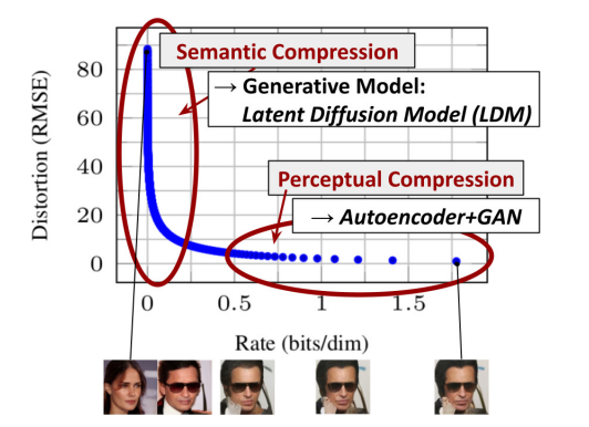
As seen above in the graph from the paper, we see the rate-distortion tradeoff. Distortion can be thought of as the root-mean-squared error (RMSE) between the original input image and the final generated image from the decoder. The lower the distortion, the lower the root-mean-squared error between the original image and the generated image. One may erroneously assume that a low distortion would always mean good perceptual quality of the image, but this is actually the complete opposite- optimizing one will alway come at the expense of another.

Rate, or bits per dimension or pixel, can be thought of as the amount of information. Therefore, higher the rate, the more "information" there is in the image. I believe that the diagram shows the progression of the reverse diffusion process, where it starts at high distortion and zero rate (completely noised image) at time T, and where it ends at low distortion and high rate (completely denoised image) at time 0. Thus, it makes sense why distortion would decrease when rate is increased, as shown in the graph. The graph above first shows the separately trained universal autoencoder for an effective mapping of the input image in the pixel space to the latent space. Therefore, this autoencoder allows the reverse diffusion process of the conditioned U-Net to focus on generating the semantic details for semantic compression.

But one may ask, why specifically use U-Net? The authors believe that by using U-Net, they can utilize the inductive bias of U-Net to generate high quality images. This is indeed true, as U-Nets, like other convolution-based networks, naturally excel at capturing the spatial relationship of images and have unique advantages like translational invariance due to convolutions.

Therefore, the authors state that their work offers three main advantages over other previous diffusion models or any general generative models:

• Training an autoencoder that maps pixel to latent space makes the forward and reverse diffusion process computationally efficient with minimal losses in perceptual quality.
• The autoencoder only needs to be trained once and then can be used for various downstream training of multiple, multi-modal generative models.
• By utilizing the image-specific inductive bias of U-Net, the model does not need aggressive compression of images which could deteriorate perceptual quality of generated images.

Before looking at experiments and results the authors concluded to verify those claims above, let’s look at the overall model architecture first.

Model Architecture:

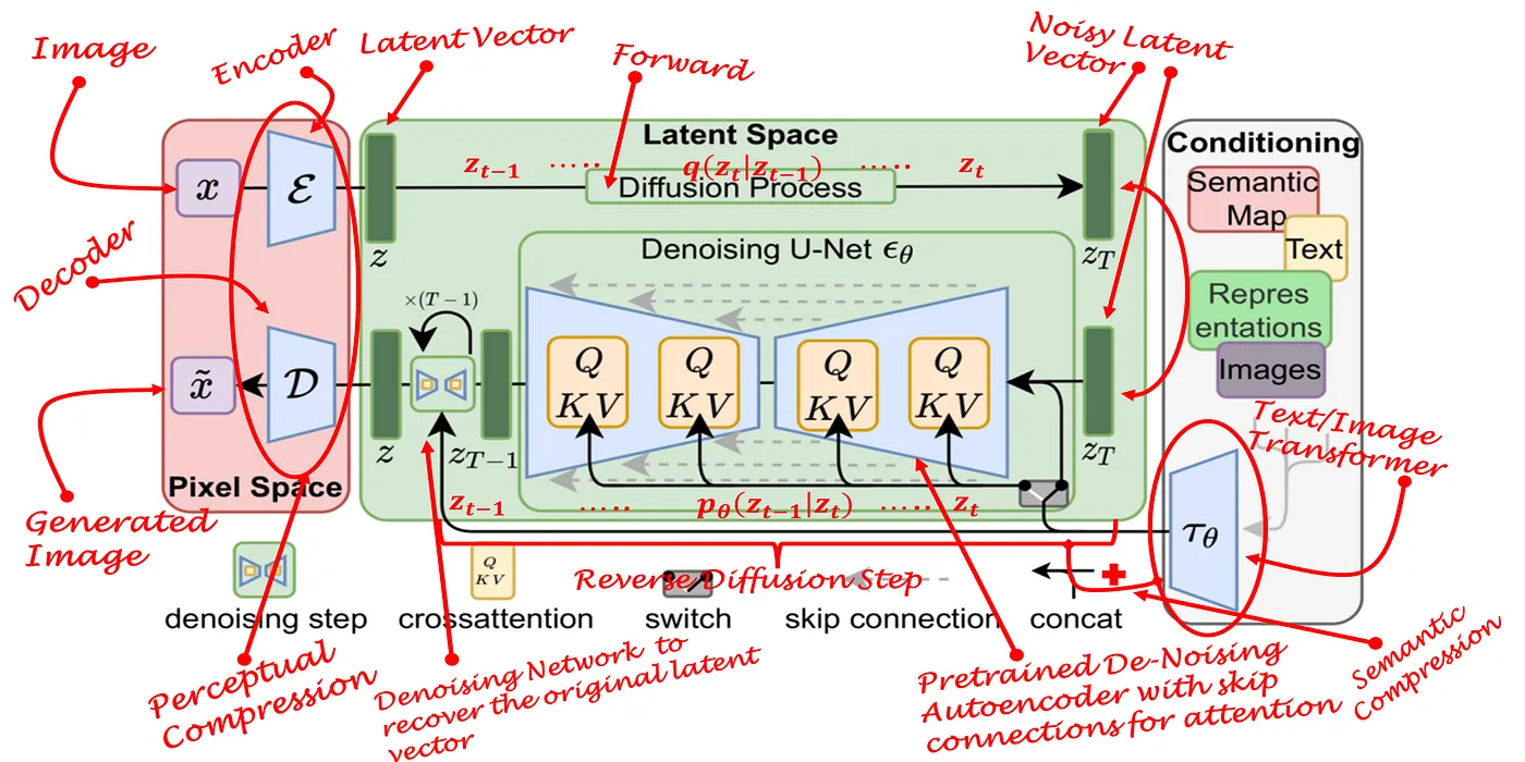
Stable diffusion consists of three major components- an autoencoder, a U-Net, and a pretrained encoder. Each of the three components are critical and work together to work their magic. The entire model architecture and its three major components can be visualized in the below image:

1. Autoencoder: The autoencoder is responsible for two major tasks, with the encoder and the decoder being responsible for each task. First, the encoder allows the previously mentioned forward diffusion process to happen in the latent space. This means that the forward diffusion process, which is Markovian, would take less time since the image from our pixel space is essentially downsampled into the latent space. Without the encoder, the forward diffusion process in the pixel space would simply take too long. Likewise, the decoder is then responsible for upsampling the generated latent space image back to the pixel space. The generated latent space image is obtained from the output of the U-Net, which will be mentioned next. The decoder is needed because the generated latent space image needs to be converted back to the pixel space to obtain our final desired image. Basically, the autoencoder allows the forward and the backward diffusion process to happen in the latent space, and also performs perceptual compression by removing high-frequency details as explained in the previous section. Note that this autoencoder can be separately trained only once and be applied in various different tasks since the generative power of the model resides in the U-Net + pretrained encoder.

2. U-Net: The U-Net, which is a popular model used in semantic segmentation, is a U-shaped fully convolutional neural network. It follows a U-shape because of its downsampling contracting path with max-pooling and its upsampling expansive path, with skip connections between each layers to preserve semantic details. The U-Net in stable diffusion, is responsible for denoising the noisy latent vector that was produced by the encoder, meaning that it is responsible for the reverse diffusion (generation) process. Therefore, when we train a diffusion model, we’re essentially training the denoising U-Net. However, this denoising U-Net isn’t without additional help, as it is conditioned by not only the noisy latent vector, but also by the latent embeddings generated by the encoder via a cross-attention mechanism built in to the U-Net architecture. Since it is a cross-attention mechanism, these embeddings can be from different modalities such as text, image, semantic map, and more. The inductive bias of the U-Net giving it a natural advantage in handling image data with cross-attention in the backbone makes the generative process stable (as aggressive compression is not needed) and flexible (cross attention allows multi-modality).

3. Pretrained Encoder:
   Therefore, the pretrained text/image (mostly text and image modalities are used as prompts) encoder is responsible for projecting the conditioning text/image prompts to an intermediate representation that can be mapped to the cross-attention components, which is the usual query, key, and value matrices. For example, BERT or BERT-like pretrained text encoders have been pretrained on huge corpus datasets and are suited to take text prompts and generate token embeddings which are the intermediate representations that gets mapped to the cross-attention components. Nowadays, CLIP or CLIP-like pretrained text/image encoders pretrained on huge dataset of image-text pairs are used and thus allows text and image prompted stable diffusion as well (BERT can not handle images).

Experiments & Results:

Now, with the above motivation resulting in the authors designing this unique model architecture, the authors performed several experiments to verify their claims.

1. Experiment on Perceptual Compression Tradeoffs:

Recall that the autoencoder is responsible for mapping the input image from the pixel space to the latent space and vice versa, and therefore needs an optimized downsampling factor for it to be effective- too high of a downsampling factor will be too aggressive in the perceptual compression and cause information loss and too low of a downsampling factor will make the training process slower since it would leave most of the perceptual compression to the reverse diffusion process (image not compressed enough). As expected, the graph below shows that a downsampling factor of 4 or 8 was the ideal factor for training the autoencoder.

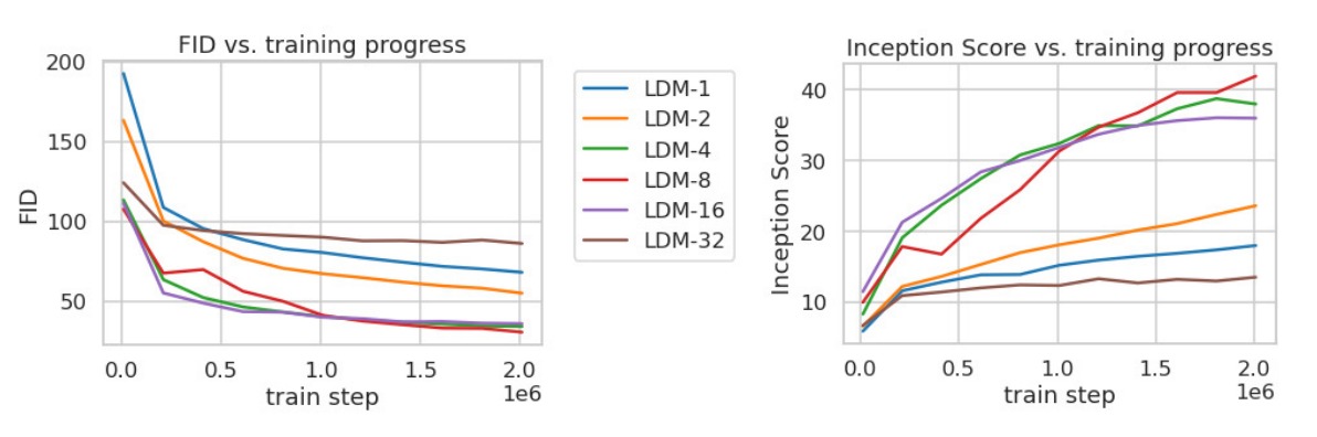
It is confirmed that LDM with downsampling factor 4 and 8 achieve the lowest FID score and the highest Inception Score, with downsampling factors at each extreme ends (1 and 32) performing poorly as expected. Lastly, the authors utilized LDM with downsampling factor of 4 and 8 and tested them against multiple benchmark datasets. It was concluded that LDM's did show SOTA performance compared to that of previous diffusion-based SOTA models in all but one dataset on FID, and also performed better than GANs on precision and recall. This improved performance was also with using significantly less computational resources, matching the author's hypothesis earlier. Please refer to the paper for more information on the results, as it is too much detail to cover every result in the blog.

2. Conditional Latent Diffusion:

Note that one of the biggest advantages to the LDM is its multi-modality due to its cross-attention based text/image conditioning made possible with the U-Net backbone and pretrained encoders like BERT and CLIP. The authors explore the multi-modality by performing different experiments in LDM's ability to perform semantic synthesis, image superresolution, and image inpainting. Before briefly looking over each experiment, however, it is important to touch upon: 1) KL and VQ-regularized LDMs and 2) Classifier-guided and classifier-free diffusion process.

-KL and VQ-regularized LDMs:
KL-regularization actually originates from variational autoencoders (VAEs), which is a type of autoencoder where its encodings are regularized so that the latent space can be sufficiently diverse, so that the resulting image generated from the decoder is diverse but also accurate. This regularization is needed because without regularization, VAEs will tend to spread out in clusters in the latent space, which deteriorates the decoder’s performance as it learns to just regurgitate the training data. This becomes more clear when looking at the below diagram:

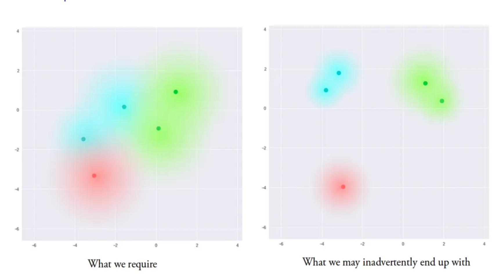
The left plot shows the VAE latent space with KL-regularization, as the clusters are closer together and each cluster has a wider "radius". This VAE will generate images that are both accurate and diverse. On the other hand, the right plot shows the VAE latent space without KL-regularization, as the clusters are further apart and each cluster has a narrower "radius". This VAE will not generate diverse images, and often times images may be "weird looking" since there is no smooth transition/interpolation between different classes (clusters are further apart).

The "KL" stands for the Kullback-Leibler (KL) divergence, that is additionally added to the loss function of the VAEs. The KL-divergence essentially measures the distance between two probability distributions, and minimizing this essentially brings the above clusters "more together". More on VAEs and KL-divergence will be covered in the next part of the blog.

VQ-regularization is another method to regularize the latent space of a VAE, a similar method is utilized in Vector-Quantized (VQ) VAEs- hence why it is called VQ-regularization. VQVAEs, unlike VAEs briefly described above, utilize discrete latent variables instead of a continuous normal distribution used in the original VAE. Then, the embeddings generated by the encoder is categorical, and samples drawn from this generate a discrete embedding dictionary. The authors call this regularization process with a "vector quantization layer by learning a codebook of |Z| different exemplars", in which the vector quantization layer converts the continuous latent distribution to discrete indices. Here, "codebook" refers to the discrete embedding dictionary. To briefly explain how the vector quantization layer works, the vector quantization works by comparing the continuous input from the encoder and the "codebook" and finding the index of the closest vector ("argmin") in the "codebook" by using Euclidean distance or other similarity measures. Again, more on VQVAEs and VQ-regularization can be covered later, but is not the focus of this blog. The authors utilize the VQ-regularization for their LDMs in the decoder of the autoencoder in an attempt to regularize the latent space, in a way to enhance the interpretability of the latent space and hence increase the robustness and quality of the generated samples.

-Classifier-guided and classifier-free diffusion process:
In the reverse diffusion or sampling process, one can utilize a classifier-guided or a classifier-free diffusion process. A classifier-guided diffusion process, like its name, requires a separate classifier to be trained. This classifier guidance technique did boost the sample quality of a diffusion model using the separately trained classifier, by essentially mixing the score (score = gradient of log probability) of the diffusion model and the gradient of the log probability of this auxillary classifier model. However, not only was training this auxillary classifier time-consuming (it requires training on noisy images, meaning it cannot be pre-trained), but this process of mixing resembles an “adversarial attack” (adversarial attack meaning introducing slight perturbations the input which confuses the model and results in different outputs). Therefore, a classifier-free diffusion process is utilized by the authors, which doesn’t require a separate classifier to be trained, and still boosts the sample quality of the LDM. This classifier-free approach requires training a conditional and an unconditional diffusion model simultaneously, and mixes the two scores together. We will look at classifier-guidance in more detail in Part 4 of the blog.

Now, to come back to the conditional LDMs, the authors wanted to test how their model performed on a text-to-image synthesis by using a BERT tokenizer. The authors concluded that their "LDM-KL-8-G" model, or their classifier-free, KL-regularized LDM with downsample factor of 8 performed on par with recent SOTA diffusion or autoregressive models despite utilizing significantly lower number of parameters. With their success, the authors tested their LDM model on four additional tasks:

-Semantic Synthesis: Semantic synthesis was tested to see the LDM’s ability to condition on different modalities outside of text. As seen in the diagram below, a 256 x 256 resolution semantic map was conditioned on the LDM to generate a 512 x 1024 resolution landscape image. The authors tested various different downsampling factors and also both KL- and VQ-regularized LDMs, and concluded that signal-to-noise ratio (SNR) significantly affected the sample quality.

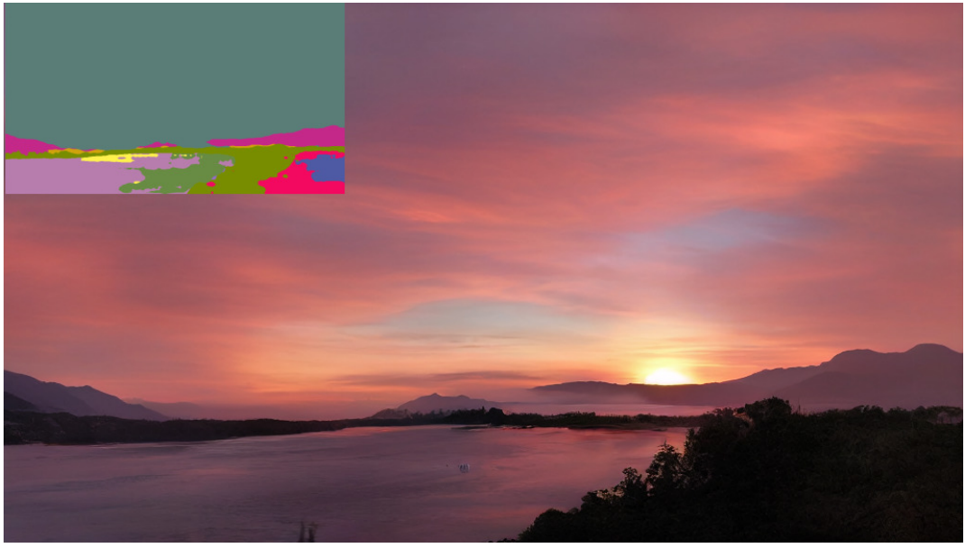
The SNR was high for LDMs trained in the latent space regularized by KL-regularization as the variance was too high- resulting in low fidelity images. Therefore, KL-regularized LDMs had its latent space rescaled by its component-wise standard deviation of the latents and the SNR was decreased (VQ-regularized space doesn’t have this issue as VQ-regularized latent space has variance close to 1).

-Image Super-resolution and Inpainting: Image super-resolution is to generate a higher resolution version of the input image, which is basically an advanced version of semantic synthesis. This was achieved by conditioning on low-resolution images as input, and those low-resolution images were initially degraded using bicubic interpolation with 4x downsampling. The LDM concatenates the low resolution conditioning and the inputs to the UNet, resulting in a “super-resolution” image. The authors were able to achieve SOTA performance, and they also developed a more general model that could handle different types of image degradation other than bicubic interpolation for robustness. Image inpainting is to fill in a masked region of a specific image. The authors also report SOTA performance on FID and noted that the VQ-regularized, 4x downsampled LDM-4 worked the best.

Most of the important parts of the paper has been covered, but there was barely any math in my explanations. Fully understanding stable diffusion without covering its mathematic details would not be possible. The next three parts (Parts 3, 4, and 5) will cover all of this.

Image credits to:

• Stable Diffusion Architecture
• VAE Latent Space KL-Regularization