(Concept Review/Generative Models) Latent/Stable Diffusion Fully Explained, Part 1
Welcome to my first blog post! From now on, I'll be trying to do regular updates on any interesting, recent AI-related topic.
For my first post, I thought it’d be fitting to do an in-depth review on the stable diffusion model which basically started the stable diffusion boom last year. It really is the “hot topic” right now, as the generative models are taking over the AI industry. For reference purposes, the stable diffusion paper that started it all is named “High-Resolution Image Synthesis with Latent Diffusion Models”, and can be found here. For this part (part 1), I will just touch upon the surface about stable diffusion and its predecessor, GANs. The next three parts, as seen in the table of contents below, will cover much more qualitative and quantitative details. Let’s dive right in!

Table of Contents:
Latent/Stable Diffusion Fully Explained! (Part 1) (This Blog!)
Latent/Stable Diffusion Fully Explained! (Part 2)
-
Motivation
-
Model Architecture
-
Experiments & Results
Latent/Stable Diffusion Fully Explained! (Part 3)
-
VAEs and ELBO
-
Model Objective
Latent/Stable Diffusion Fully Explained! (Part 4)
-
Different View on Model Objective
-
Training and Inference (DDIM vs DDPM)
Latent/Stable Diffusion Fully Explained! (Part 5- Coming Soon!)
-
Conditioning
-
Classifier-Free Guidance
-
Summary
Note: For other parts, please click the link above in the table of contents.
Background:
Latent diffusion models (LD), or henceforth mentioned as stable diffusion models (SD), are a type of a diffusion model developed for the purpose of image synthesis by Rombach et al. of last year. (While LD and SD are not exactly equal- SD is an improved version and hence a type of LD- we will use the term interchangeably) Let’s do a quick review/introduction of what a “model” is first:
Introduction:
In Machine Learning, a model is either a generative or discriminative. The diagram below clearly shows the difference between the two:
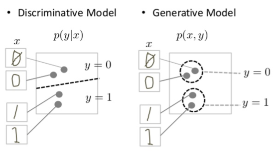
As shown above, the discriminative model tries to tell the difference of a writing of 0 and 1 by just simply drawing a decision boundary through the data space. Therefore, a discriminative model just has to model the posterior \(p(y|x)\) for label y and data sample x. It doesn’t need to model the probability distribution of the entire data space to do this. For example, if you are familiar with SVMs, which is a type of a discriminative classifier/model, we know that the model’s objective is to find the support vectors that maximize the distance between the support vectors and the decision boundary, which is the margin. Most of the time, the support vectors are very few data points that lie near the decision boundary (hyperplane)– the majority of the other data samples simply don’t matter.
On the other hand, a generative model aims to model the probability distribution \(p(x,y)\) of the entire data space. For cases where there is no label (semi-supervised/unsupervised cases), a generative model aims to model \(p(x)\) instead. We can see in the diagram above that the generative model has come up with a probability distribution of the 0’s and the 1’s that well-represents the true, hidden probability distribution of the entire data space. Therefore, the generative model generally has to “work harder” to achieve its goals. However, this unique nature of generative models allows it to “generate” synthesized data by using sampling methods from the modeled probability distribution, just like the cute pikachu drawing I generated by using DALLE-2, which is a type of generative model! Likewise, a stable diffusion model is a type of generative model. Generative models can be broadly classified into four types:
- Flow-based models: Flow-based generative models are quite unique in that they utilize a method called “normalizing flow”. Normalizing flow uses the change of variable theorem, which allows us to estimate a more complex probability density function for our model. This is hugely beneficial but also comes at a cost- during backpropagation, the derivative would be impossible or too hard to calculate. Therefore, we will later see that this is why stable diffusion utilizes the gaussian distribution in its noising process, even though it is much simpler than the “real world” distribution. Normalizing flow is essentially a complex distribution modeled by a chain of invertible transformation functions. The probability density function is tractable, meaning the learning process is simply based on minimizing the negative log-likelihood over the given dataset. A critical drawback, however, is that normalizing models have limitations in that the transformations must all be invertible (for change of variable theorem to work) and determinants must be efficiently calculated (for backpropagation).
- Autoregressive models: Autoregressive generative models, like their name suggests, means performing regression on its self. General autoregression means predicting a future outcome based on the previous data of that outcome. The general idea is that autoregressive models model the joint probability space \(p(x)\) by utilizing the chain rule \(p(x,y) = p(y|x)p(x)\), meaning that it is ultimately a product of conditional distributions. Like normalizing flows, defining the complex product of conditional distribution is no easy task, and autoregressive models do this by utilizing the deep neural networks. In this case, outputs of the neural network is fed back as input, with the layers being one or more convolutional layers. Like normalizing flow models, the probability distribution is tractable, but the sampling process is slower as it is sequential by nature (sequential conditionals).
- Generative Adversarial Networks (GAN): GANs will be covered in more detail in this blog.
- Latent variable models: Stable diffusion models belong to this type. This will also be covered in more detail in this blog.
Why ditch GANs for Stable Diffusion?
Surprisingly, diffusion models are not new at all! Stable diffusion is a type of diffusion model, and like its name suggests, is actually based on the diffusion from thermodynamics! The forward diffusion process is where random (usually Gaussian) noise is introduced to an image until the image is pure noise (isotropic Gaussian), and the reverse diffusion process is where the model is trained so that the model is able to generate data samples from the noise that is representative of the true data distribution. Before diving deeper into stable diffusion, let’s first review GAN’s disadvantages, because before stable diffusion’s emergence as the SOTA (state-of-the-art) generative model, GAN and its variants have been the SOTA generative model (however GANs still may be superior in niche use cases since sampling is still much faster on GANs).
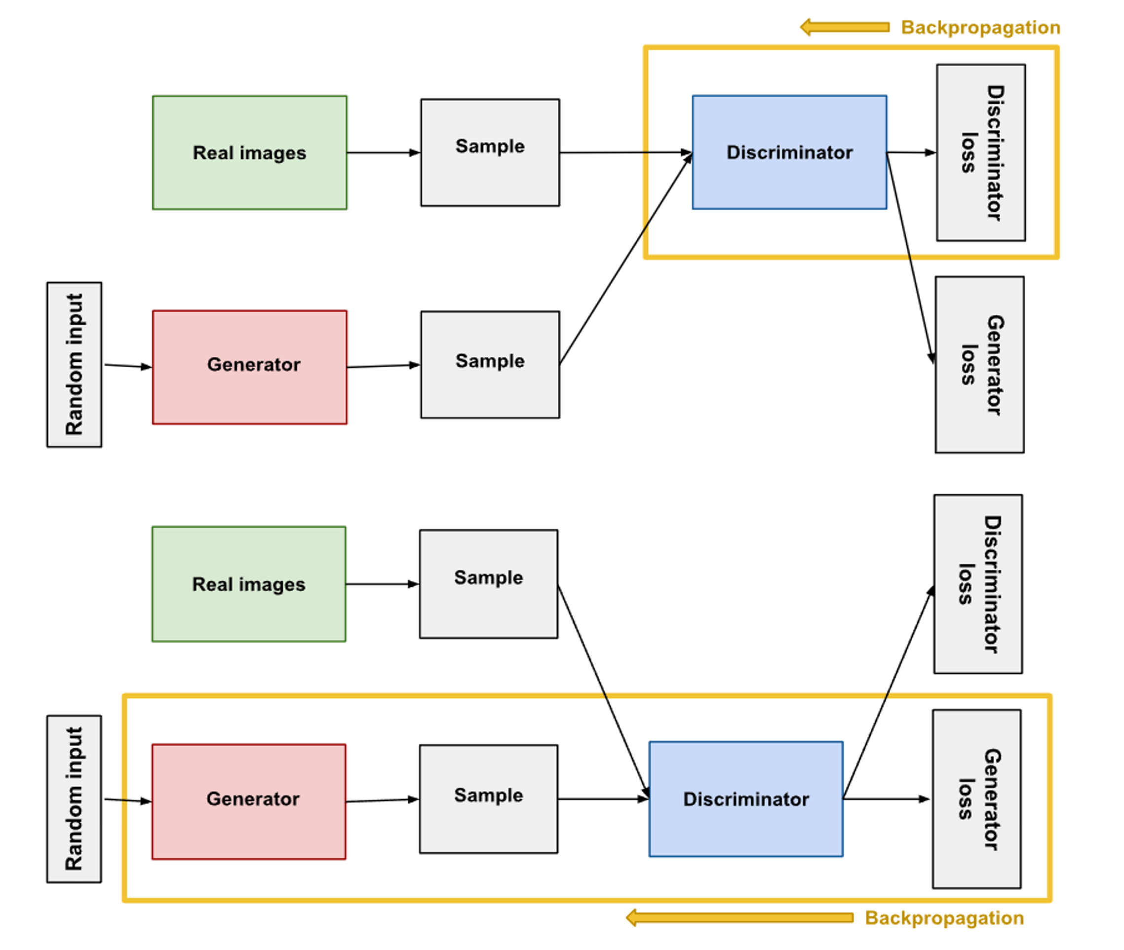
The diagram above shows the general GAN architecture. As seen in the diagram, a GAN consists of a generator and a discriminator, which are both deep neural networks that are trained. The generator learns to generate plausible data, or so-called "fake images". The generated instances of fake images then become negative training examples for the discriminator. Then, the discriminator learns to distinguish the generator's fake data from real data. Hence, the discriminator is simply a classifier model where it labels the images generated by the generator as real or fake. Simple!
The training process consists of the discriminator loss penalizing the discriminator for misclassifying the real image as fake or fake image as real. Then, the suffered loss is then used for backpropagation to update the discriminator’s weights. Next, the generator takes a random input of noise, which is a probability distribution (e.g. Gaussian) and generates the fake samples. The training process consists of the generator loss penalizing the generator for not being able to "trick" the discriminator. Likewise, the suffered loss is used for backpropagation to update the generator’s weights. Note that the discriminator and generator are separately trained, meaning that when the generator is trained the weights of the discriminator is fixed.
The ideal situation is that if this is done repeatedly, the generator would eventually be able to learn the entire joint probability distribution of the desired data set. But how do we know if we’re done training? This is one of GAN’s biggest drawbacks, but generally, if the discriminator is starting to give completely random feedback, we know we’ve done well. This would mean that the generator is generating fake images that are so similar to the real images that the discriminator cannot distinguish them. Now let’s touch upon the critical disadvantages that GANs have due to their intrinsic architecture and training approach.
- GANs are a type of implicit generative model, meaning it implicitly learns the joint probability distribution (probability density function is intractable), meaning that any modification or inversion of the model is difficult. (Explicit generative models like the flow-based and autoregressive models have tractable density functions.) This makes training unstable, as we cannot rely on the actual loss function of the GAN during the training process.
- Furthermore, because two separate networks must be trained, GANs suffer from high training time and will sometimes fail to converge if GAN continues training past the point when the discriminator is giving completely random feedback. In this case, the generator starts to train on junk feedback, and the generated image will suddenly start to degrade in quality.
- Also, if the generator happens to create a very plausible output, the generator in turn would learn to only produce that type of one output. If the discriminator then gets stuck in a local minima and it can’t find itself out, the generator and the entire model only generates a small subset of output types. This is a common problem in GANs called mode collapse.
- Lastly, we can have vanishing gradients when the discriminator performs very well, as there would be little loss suffered from the generator and hence almost no weight updated for the generator model through backpropagation.
To address these issues during training, when training and evaluating GANs, researchers generally use both qualitative and quantitative metrics during the training and evaluation process. Qualitative metrics are essentially human judges rating the quality of the generated images compared to the ground-truth images. Quantitative metrics that are often used, are Inception Score (IS) and Frechet Inception Distance (FID).
While the drawbacks of GANs listed above do have their own remedies, they may still not work, or even if they do work, they may require a lot of time and effort- which may not be worth it. However, stable diffusion hasn’t become the SOTA generative model just because of the drawbacks of GANs, they have their own advantages as well! The paper itself will be detailed in part 2.
Image credits to: