(Concept Review/Segmentation Models) How to use Class Activation Maps (CAM) for Explainable AI in Semantic Segmentation
In this post, I will briefly describe Class Activation Maps (CAM) and some of its popular subtypes, usages in semantic segmentation, and then finally post some code and results in utilizing CAM in my own semantic segmentation project using H&E images.
Table of Contents:
-
What are Class Activation Maps (CAM)?
-
CAMs in Image Semantic Segmentation:
-
Utilizing CAM in My Project
What are Class Activation Maps (CAM) ?
Class activation maps, henceforth referred to as CAM, can be thought of as heatmaps that can highlight the regions of a query image that are most important for the network’s classification or segmentation decision. Before introducing CAMs, why do we want to look at CAMs in the first place?
CAMs are probably one of the most popular and easy-to-do explainable AI metrics, which aim to understand and interpret the decisions made by built machine learning models. Let’s come up with an example where CAMs would be useful: Let’s say I work for a AI company and we built a machine learning model that looks at a chest x-ray and is able to detect a rare disease that occurs 1% of the time with 99% sensitivity (so the model itself is sensitive (or has high recall), so it isn’t saying no all the time and has 99% accuracy). However, by utilizing CAMs before deploying the model, I find out that the model is actually only looking at a circle at the corner of the x-ray image to detect the rare disease. Upon checking the images used for training/validation/testing, they all had a circle at the corner that the hospital used to specify that this was a positive image. Without CAMs, we would have no idea this was the case and would’ve been deploying a completely useless model!
Like the above made-up example, traditionally, CAMs were developed to be used for image classification, as utilization of CAM was limited to specific types of architectures, which are CNNs with global average pooling (GAP) and a final fully connected layer. Most image classification models use GAP and a final fully connected layer followed by the output activation function (assume multi-class, so we use softmax) for turning logits into final prediction probability/results. The last layer before the GAP and fully connected layer is the layer that holds the “feature map”, which captures subtle, fine semantic details of the training images. The implementation of CAM is beautifully summarized in the diagram below:
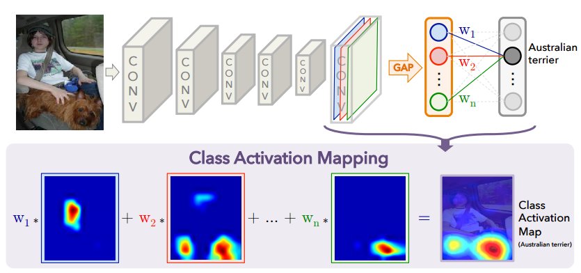
As seen in the above diagram, the class activation map is generated by a linear combination of all the \(n\) weights (weights in the fully connected layer) for the specific class (in the above case, the Australian terrier) and all the \(n\) feature maps. For example, in the diagram above, we can tell that \(w_2\) would have a higher weight than \(w_1\) since the feature map \(F_2\) has to do with the Australian terrier. Mathematically, the CAM can be represented as:
$$Y_c = \sum_{k} {w_k}^{c} \cdot \frac{1}{Z} \sum_{i}\sum_{j} A_{(i,j)}^{k}$$ $$Y_c = \sum_{k} {w_k}^{c} \cdot F^{k} \quad (1)$$
,where \(Y_c\) is the activation score (CAM) for \(c\), which is the specific class (like Australian terrier). \(k\) is the number of feature maps and therefore \({w_k}^{c}\) is the weight for \(k\)th feature map for class \(c\). Lastly, \(A_{(i,j)}^{k}\) is the \(k\)th feature map for pixel coordinate \((i,j)\), which is summed over all \(i\) and \(j\) and divided by total number of pixels \(Z\) to return our global average pooled feature map \(F^{k}\). We can see that \(\frac{1}{Z} \sum_{i}\sum_{j}\) is the mathematical representation of global average pooling (GAP). Finally, since feature maps are downsampled compared to the original image size, we need to perform bi-linear interpolation on the CAM to upsample for us to visualize the overlay of the CAM on the query image like shown in the diagram above.
However, as mentioned above, the general CAM method requires an architecture that includes all of the three:
- A feature map, or the penultimate layer of the model.
- A global average pooling operation to the feature map.
- A final fully connected layer followed by an activation function to produce prediction labels.
Since not all methods satisfy all three requirements above, CAM was only limited to certain types of architecture, making it unavailable to use for other types of CNN architectures that are dense like VGG, handle multi-modal inputs/perform reinforcement learning.
CAMs in Image Semantic Segmentation:
As mentioned previously, the three requirements for CAM severely limited the usage to certain types of architectures, and was totally not applicable for non-CNN based models such as vision transformers, or ViTs (to be fair, when CAM was first released, transformers were not a thing yet). Therefore, GradCAM, or Gradient-weighted CAMs, were widely used which essentially replaces the weights of the fully connected layer with calculated gradients that flow back into the last convolutional layer. To show that this is true, consider taking the gradient of the activation score for class \(c\) (\(Y^{c}\)) with respect to feature map \(F^{k}\) from the above CAM equation, or equation #1:
$$ Y_c = \sum_{k} {w_k}^{c} \cdot F^{k}$$ $$\frac{\delta Y^{c}}{\delta F^{k}} = \frac{\frac{\delta Y^{c}}{\delta A_{(i,j)}^{k}}} {\frac{\delta F^{k}}{\delta A_{(i,j)}^{k}}} $$ $$\text{Recall from above: } F^{k} = \frac{1}{Z} \sum_{i}\sum_{j} \text{ so: } \frac{\delta F^{k}}{\delta A_{(i,j)}^{k}} = \frac{1}{Z}$$ $$\text{Then: } \frac{\delta Y^{c}}{\delta F^{k}} = \frac{\delta Y^{c}}{\delta A_{(i,j)}^{k}} \cdot Z $$ $$\text{Recall from above: } Y_c = \sum_{k} {w_k}^{c} \cdot F^{k} \text{ so: } \frac{\delta Y^{c}}{\delta F^{k}} = {w_k}^{c}$$ $$\text{Then: } {w_k}^{c} = Z \cdot \frac{\delta Y^{c}}{\delta A_{(i,j)}^{k}} \quad (2)$$
Now note that above equation #2 is only for pixel location \((i,j)\), so let’s sum over all pixels. Note that \(\sum_{i}\sum_{j} 1 = Z\):
$$\sum_{i}\sum_{j} {w_k}^{c} = Z \sum_{i}\sum_{j} \frac{\delta Y^{c}}{\delta A_{(i,j)}^{k}}$$ $$Z{w_k}^{c} = Z \sum_{i}\sum_{j} \frac{\delta Y^{c}}{\delta A_{(i,j)}^{k}}$$ $${w_k}^{c} = \sum_{i}\sum_{j} \frac{\delta Y^{c}}{\delta A_{(i,j)}^{k}} \quad (3)$$
The equation #3 is an important result, this shows us that the weights for feature map \(k\) for class \(c\) are equal to the gradient of the activation score with respect to the \(k\)th feature map. But remember, we’re no longer using the weights of the fully connected layer! By re-introducing the normalization constant \(1/Z\) for global average pooling, and pooling over the gradients instead, we obtain neural importance weights \(\alpha_k^{c}\) instead:
$${\alpha_k}^{c} = \frac{1}{Z} \sum_{i}\sum_{j} \frac{\delta Y^{c}}{\delta A_{(i,j)}^{k}} \quad (4)$$
We can think of this neural importance weight \({\alpha_k}^{c}\) as the equivalent to the \({w_k}^{c}\) in vanilla CAMs. Therefore, use equation #1 for CAM above and sum over all \(k\) feature maps to find our equation for evaluating our activation score for Grad-CAM:
$$Y_c = \sum_{k} {\alpha_k}^{c} \cdot F^{k} \text{ where } {\alpha_k}^{c} = \frac{1}{Z} \sum_{i}\sum_{j} \frac{\delta Y^{c}}{\delta A_{(i,j)}^{k}} (5)$$
Equation #5 is one-step short of completion. Why? The gradients can be negative or positive! We are only interested in finding features that have a positive influence on class \(c\). This means that the activation score should be positive, and to have a positive gradient, the feature map should be positive as well. Therefore, with Grad-CAM we can highlight regions in the image, or features, that contribute to increasing the class activation score. On the other hand, negative gradients most likely belong to features in the image that are correlated with classes that are not \(c\), and therefore we apply ReLU function to suppress negative gradients and only keep positive gradients:
$$Y_c = ReLU (\sum_{k} {\alpha_k}^{c} \cdot F^{k}) \text{ where } {\alpha_k}^{c} = \frac{1}{Z} \sum_{i}\sum_{j} \frac{\delta Y^{c}}{\delta A_{(i,j)}^{k}} (6)$$
Equation #6 above is the final equation for Grad-CAM. Now, even though CAMs were widely used for classification, they could definitely also be used for semantic segmentation tasks where each pixel is labeled as a class. In this case, however, we have to modify equation #6 a bit. This is because image classification outputs a single class distribution (ex. this image is a dog), image semantic segmentation doesn’t, as it outputs logits for every pixel \((a,b)\) predicted for class \(c\). Therefore, it makes sense to sum all of these pixels as the activation score so that it becomes a single class distribution like image classification. We therefore modify the \(Y^{c}\) in the gradient to \(\sum_{(a,b) \in M}{Y_{(a,b)}}^{c}\) where \(M\) is a set of all pixel indices that belong to class \(c\) in the segmentation prediction. The final equation for Grad-CAM in image segmentation is shown below:
$$Y_c = ReLU (\sum_{k} {\alpha_k}^{c} \cdot F^{k}) \text{ where } {\alpha_k}^{c} = \frac{1}{Z} \sum_{i}\sum_{j} \frac{\delta \sum_{(a,b) \in M}{Y_{(a,b)}}^{c}}{\delta A_{(i,j)}^{k}} (7)$$
However, if we look at the equation #6 or #7 above for Grad-CAM carefully, there is a critical issue- when calculating the neural importance weight \({\alpha_k}^{c}\) the gradients are averaged due to global average pooling (GAP). Why can this be a problem? Look at the diagram below: 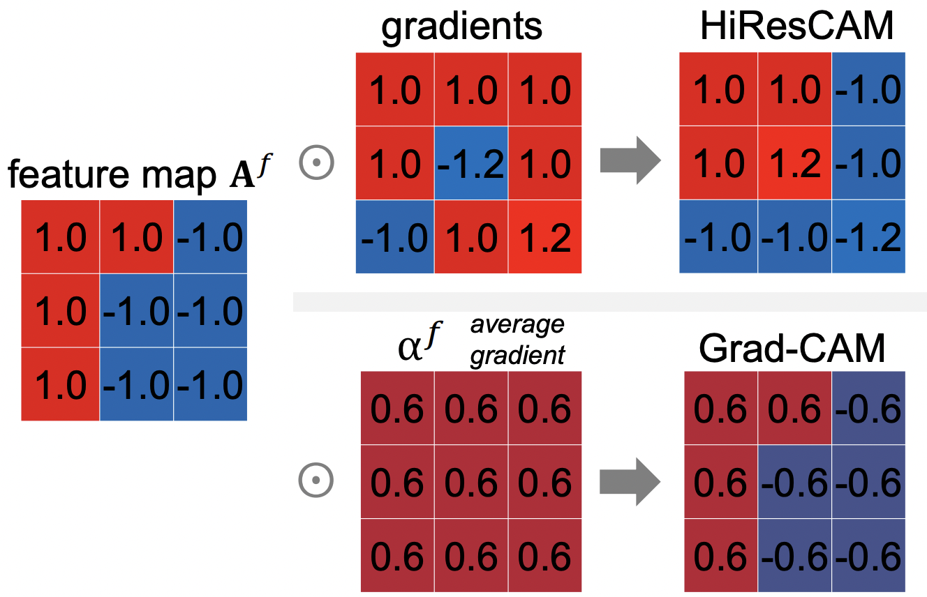
As seen in the diagram above, we see an example of a 3 x 3 feature map. Note the positive/negative pattern of this feature map. With HiResCAM, the feature map is multiplied by the gradients in an element-wise matter, and we can see that the positive and negative gradients are taken into account in the resulting HiResCAM. However, with Grad-CAM the gradients are all averaged out, and therefore the negative gradients are actually suppressed, and therefore the resulting Grad-CAM retains its original positive/negative feature map pattern. Therefore, we see that HiResCAM produces accurate attention.
Utilizing CAM in My Project:
Now that we know the differences between GradCAM and HiResCAM, below is the code that I utilized to generate CAM for my skin H&E tissue images to assess how my DeepLabv3+ image segmentation segments the classes and if it is cheating or not!
First import relevant packages, including our pytorch-grad-cam library from the official repo:
import torch
import torch.functional as F
import numpy as np
import requests
import torchvision
from PIL import Image
from torch.utils.data import Dataset, DataLoader
import cv2
import os
from natsort import natsorted
from tqdm import tqdm
from pytorch_grad_cam.utils.image import show_cam_on_image, preprocess_image
from pytorch_grad_cam import GradCAM, HiResCAM, GradCAMElementWise, ScoreCAM, GradCAMPlusPlus, AblationCAM, XGradCAM, EigenCAM, EigenGradCAM, FullGrad, LayerCAM
from pytorch_grad_cam.utils.model_targets import ClassifierOutputTarget
from pytorch_grad_cam.utils.image import show_cam_on_image
Image.MAX_IMAGE_PIXELS = None
import segmentation_models_pytorch as smp
import albumentations as A
from albumentations.pytorch import ToTensorV2
device = torch.device("cuda:0" if torch.cuda.is_available() else "cpu")
Then, write your own function to load relevant model (for me, my DeepLabV3+ segmentation model) and if necessary, your own dataloading function as well:
test_transforms = A.Compose([ToTensorV2()])  #just convert to tensor

class TestDataSet(Dataset):
    # initialize imagepath, transforms:
    def __init__(self, image_paths: list, transforms=None):
        self.image_paths = image_paths
        self.transforms = transforms

    def __len__(self):
        return len(self.image_paths)

    # define main function to read image, apply transform function and return the transformed images.
    def __getitem__(self, idx):
        image_path = self.image_paths[idx]
        image = cv2.imread(image_path, cv2.COLOR_BGR2RGB)
        image = np.array(image)
        if self.transforms is not None:  # albumentations
            transformed = self.transforms(image=image)
            image = transformed['image']
        return image # return tensors of equal dtype and size
        # image is size 3x1024x1024 and mask and bin_mask is size 1x1024x1024 (need dummy dimension to match dimension)

# define dataloading function to use above dataset to return train and val dataloaders:
def load_test_dataset():
    test_dataset = TestDataSet(image_paths=test_images, transforms=test_transforms)
    test_dataloader = DataLoader(dataset=test_dataset, batch_size=1, num_workers=0, pin_memory=True, shuffle=False)
    return test_dataloader  # return train and val dataloaders
Then write a function to return the predicted segmentation tissue map (for all classes) for the image to generate HiResCAM for:
image_path = # your own path to folder containing images to test for CAM
test_images = # complete path of the single image to test for CAM within image_path
test_dataloader = load_test_dataset()
@torch.no_grad()  #decorator to disable gradient calc
def return_image_mask(model, dataloader, device):
    weight_dir = # your own path to the saved model weights
    model.load_state_dict(torch.load(weight_dir))  #load model weights
    pbar = tqdm(enumerate(dataloader), total=len(dataloader), desc='Inference', colour='red')
    for idx, (images, image_path) in pbar:
        model.eval()  # eval stage
        images = images.to(device, dtype=torch.float)  #move tensor to gpu
        prediction = model(images)
        prediction = torch.nn.functional.softmax(prediction, dim=1).cpu() #softmax for multiclass
    return prediction
prediction = return_image_mask(model,test_dataloader,device) #predicted segmentation tissue map
Then, preprocess the image (imagenet mean/std) to generate HiResCAM for:
rgb_img = np.array(Image.open(image_path))
rgb_img = np.float32(rgb_img) / 255
input_tensor = preprocess_image(rgb_img, mean=[0.485, 0.456, 0.406],
                                std=[0.229, 0.224, 0.225]) #imagenet mean/std
Then, define a class to return the sum of the predictions of a specific chosen class (ex. class ECM for skin tissue), or the “target”.
class SemanticSegmentationTarget:
    def __init__(self, category, mask):
        self.category = category
        self.mask = torch.from_numpy(mask)
        if torch.cuda.is_available():
            self.mask = self.mask.cuda()

    def __call__(self, model_output):
        return (model_output[self.category, :, : ] * self.mask).sum()
Then, below is the most important part: For a specific chosen class (ex. class ECM for skin tissue), return the “target”, choose a layer of interest from the loaded model, choose a CAM method (we choose HiResCAM, which was explained above) and utilize pytorch-grad-cam’s functions to generate our CAM image!
he_mask = prediction[0, :, :, :].argmax(axis=0).detach().cpu().numpy()
# for skin: {"corneum" : 1,"spinosum": 2,"hairshaft":3,"hairfollicle":4,"smoothmuscle":5,"oil":6,"sweat":7,"nerve":8,"bloodvessel":9,"ecm":10,"fat":11,"white/background":12}
class_category = 6 # 6 = oil glands
he_mask_float = np.float32(he_mask == class_category)
targets = [SemanticSegmentationTarget(class_category, he_mask_float)] # return targets
target_layers = [model.encoder.layer4] # we choose last layer
with HiResCAM(model = model, target_layers = target_layers, use_cuda = torch.cuda.is_available()) as cam:
    grayscale_cam = cam(input_tensor=input_tensor,targets=targets)[0,:] # return CAM
    cam_image = show_cam_on_image(rgb_img, grayscale_cam, use_rgb=True) # overlay CAM with original rgb image
Image.fromarray(cam_image) #visualize resulting CAM
Finally, let’s look at some examples of CAMs for some of my skin H&E tissue images, and hopefully we’ll see that my trained model is actually focusing on the right parts of the images and not cheating!


The left images are GradCAMs, and the right images are HiResCAMs Now let’s analyze the images of each row. The first row are the CAMs for the background, and we can see that there isn’t a big difference between the two, except that HiResCAM does show a more “accurate” depiction, as it is a faithful explanation after all. The second row are the CAMs for the blood vessels, and we can see that HiResCAM also has a more “accurate” depiction while GradCAM shows activation scores for spots that are not blood vessel-specific. Lastly, the third row are the CAMs for the oil glands, and this is where GradCAM is a bit misleading. GradCAM does highlight the oil glands successfully, but when looking at HiResCAM, we can see that the model doesn’t only look at oil glands. Therefore, with HiResCAM, I can see that the model is also mostly looking at nearby ECM and hair follicle areas for segmenting oil glands, which is quite interesting.
The last example like above is the reason why we must continue to explore and try different types of CAMs, and also explore other options of explainable AI as well. Hope this helps!
Image credits to: